Part 1.1: Convolutions from Scratch
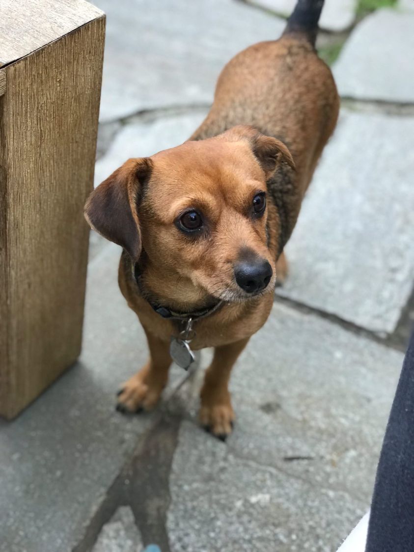
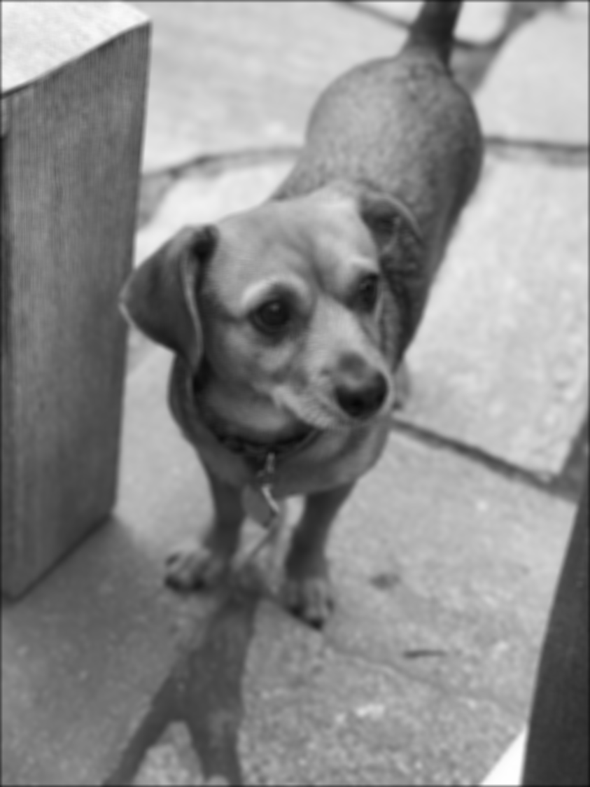
In this part, we test out different convolution approaches: one using 4 for-loops, one using 2 for-loops (slightly vectorized), and convolve2d from scipy. Overall, convolve2d was much faster than the naive implementations above. Convolving a box filter with an image of my friend's dog took well over a minute with the 4 for-loop implementation (~1 min 15 sec), 10 seconds with the vectorized convolution, and was nearly instantaneous with convolve2d (< 1 sec). By inspection, the results also looked identical as the boundaries and edges were pretty much the same.
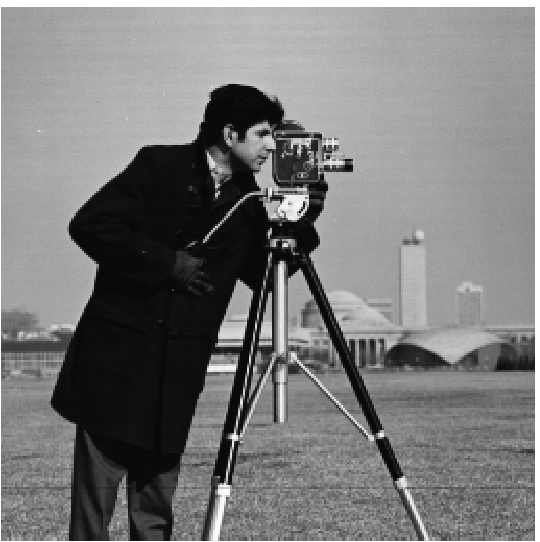
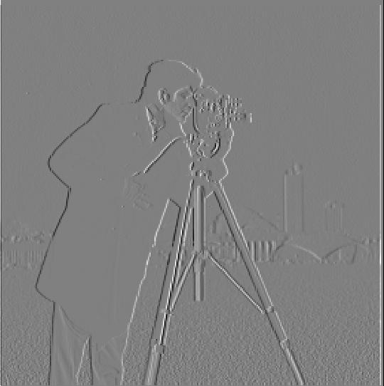
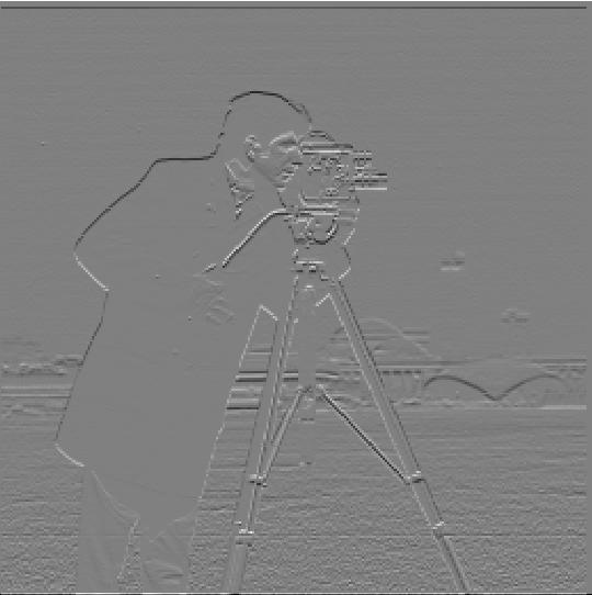
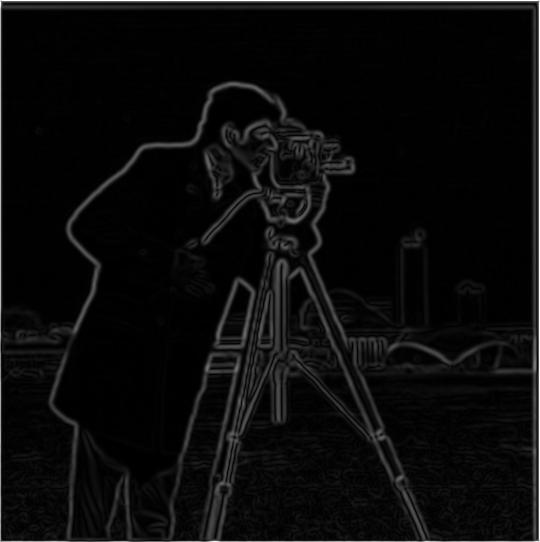
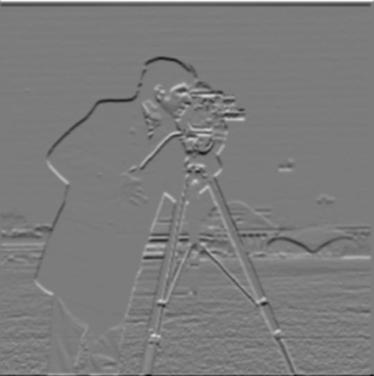
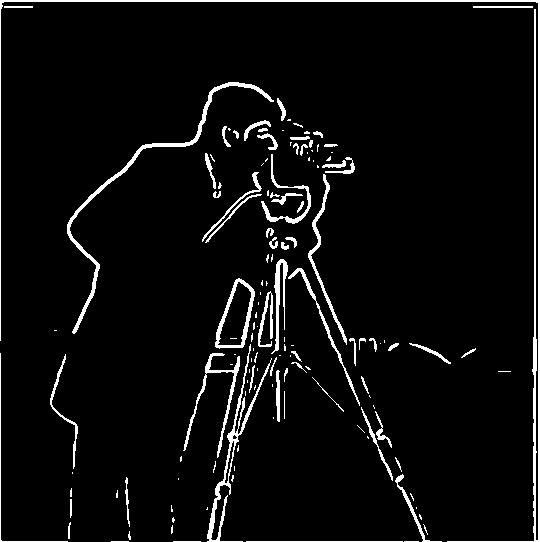
Part 1.2: Finite Difference Operator
In this part, we test out the finite difference operators and try to find an optimal threshold value that detects edges in our images while ideally minimizing noise. After trying out different threshold values, I decided to go with a 0.25 threshold as the image was still noisy when using a 0.2 threshold whereas at 0.3, the edges started to disconnect.
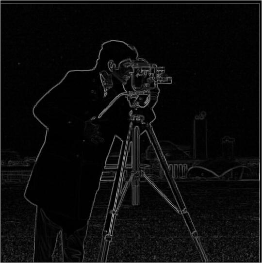
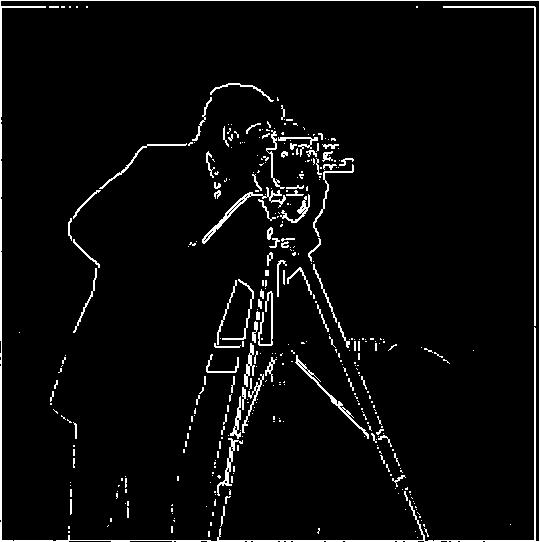
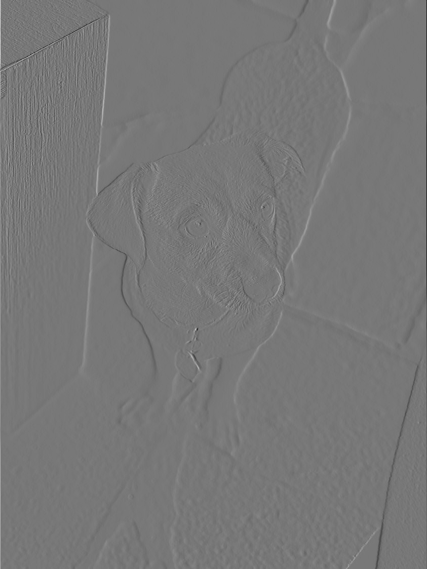
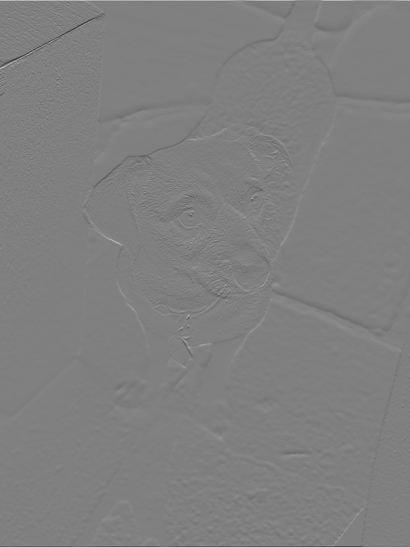
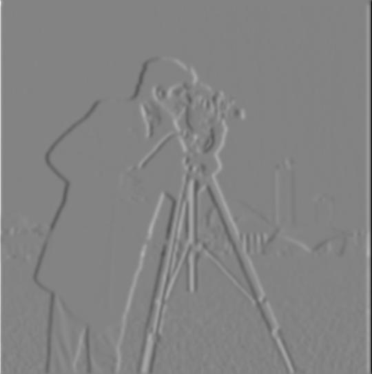
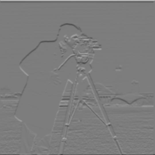
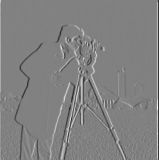
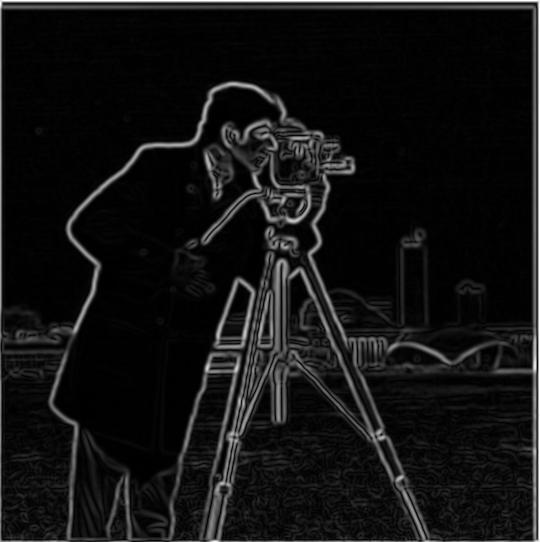
Part 1.3: Derivative of Gaussian (DoG) Filter
In this part, we try a different approach to edge detection by convolving with a Gaussian filter instead of applying finite of difference operators directly, allowing us to produce much smoother edges albeit with a higher threshold value (I used a threshold of 40 here). We tried two different approaches: (1) we apply a Gaussian filter on images before taking their derivative and convolving, (2) we convolve Gaussian filters with derivatives then apply on images. Both produced the same, smoother result compared to part 1.2. A kernel size of 9 was applied on these images.


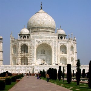
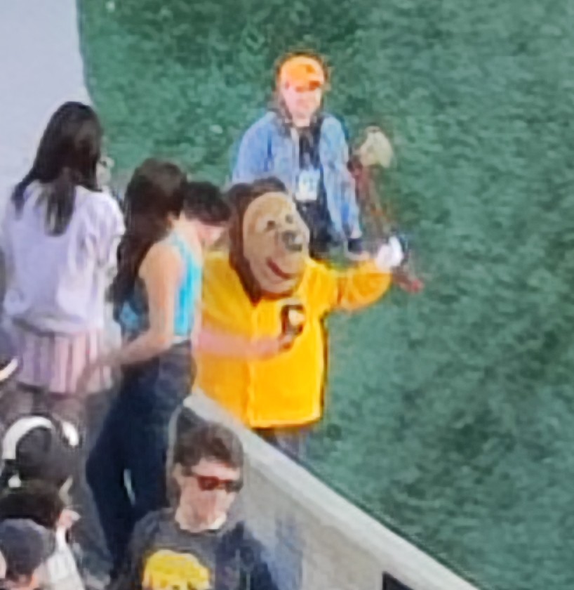
Part 2.1: Image "Sharpening"
Next, we use a masking technique to "sharpen" an image. This is done by getting the high frequences of the image (subtracting the blurred image from the original), scaling it by some alpha value, and adding it back to our original image. I tested the technique on an image of the Taj Mahal as well as a super blurry image of Oski along with different alpha values.
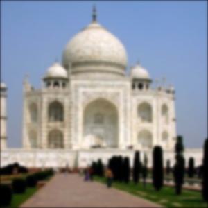
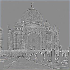
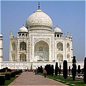
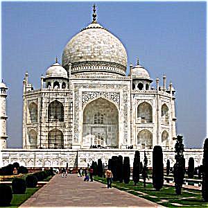


I also tried blurring then re-sharpening a sharp image and it looked comparable to the original one, although the colors were slightly less vibrant in the sharpened version.
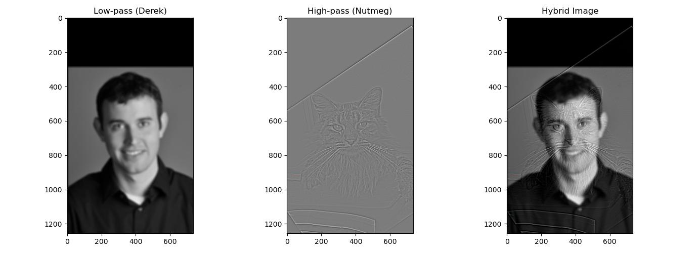
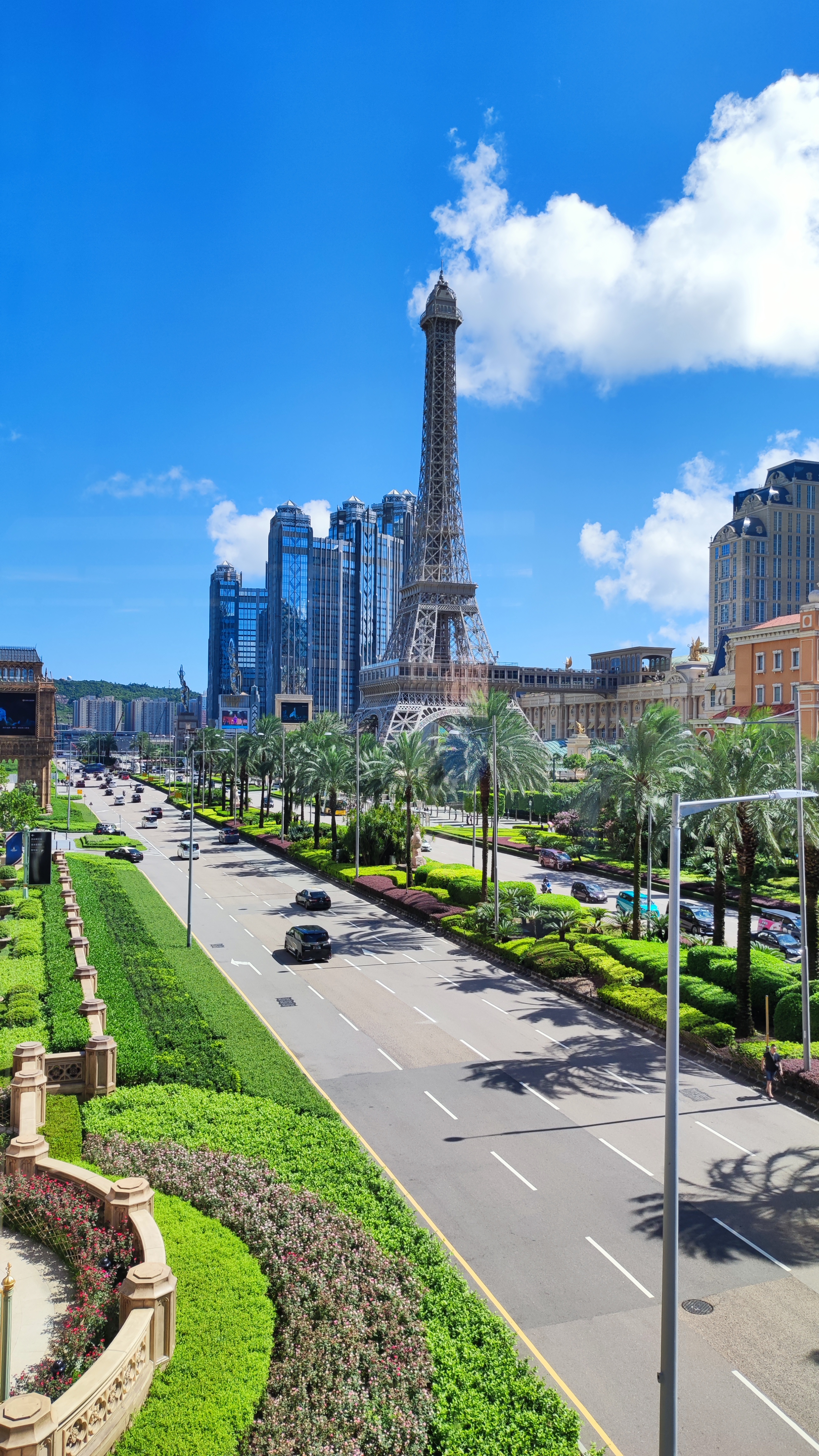
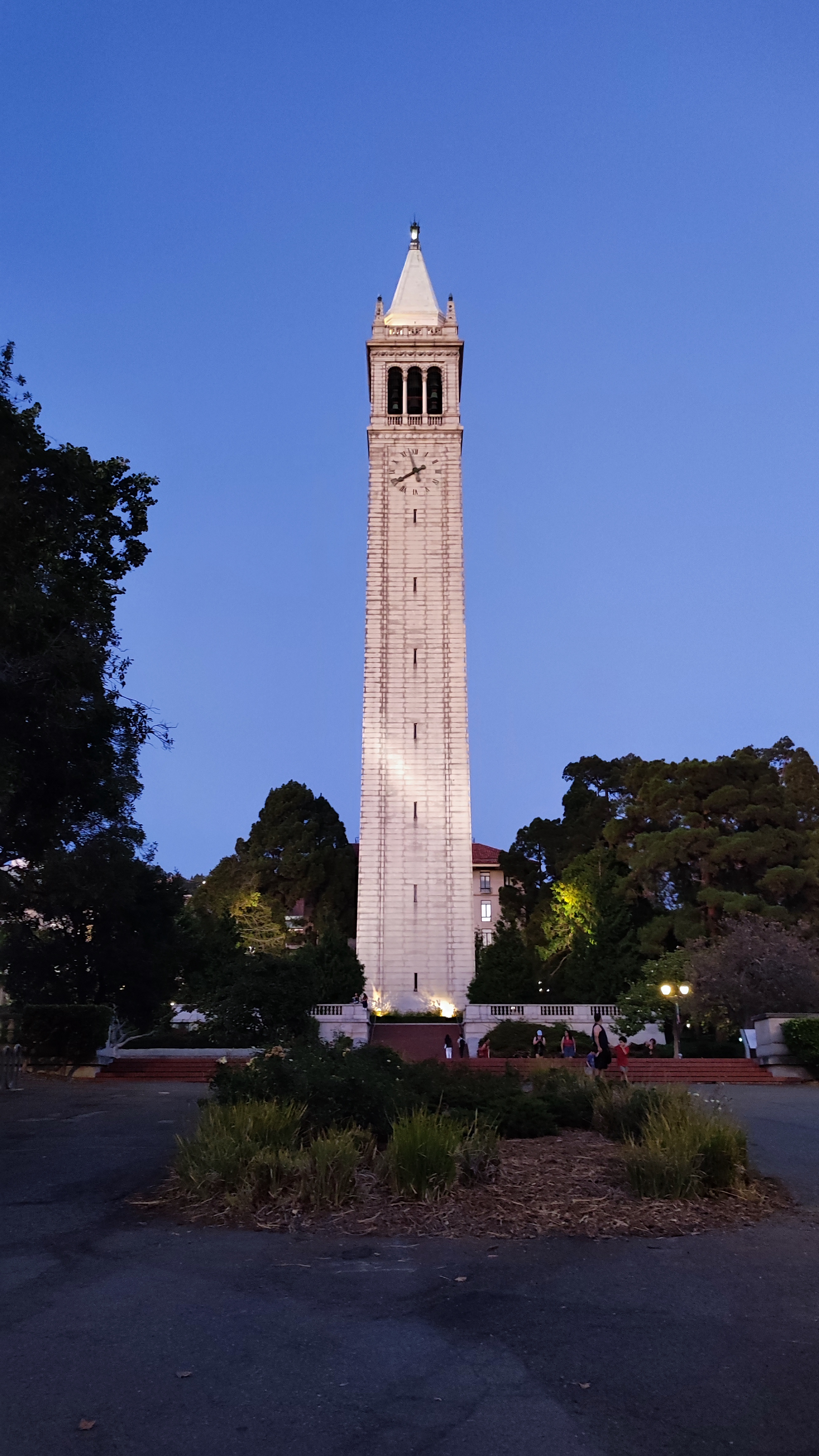
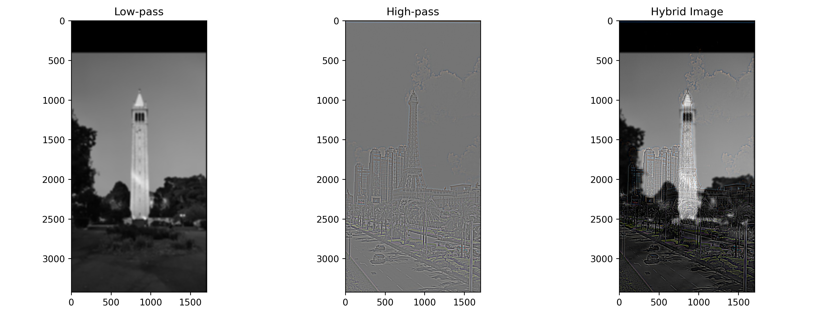
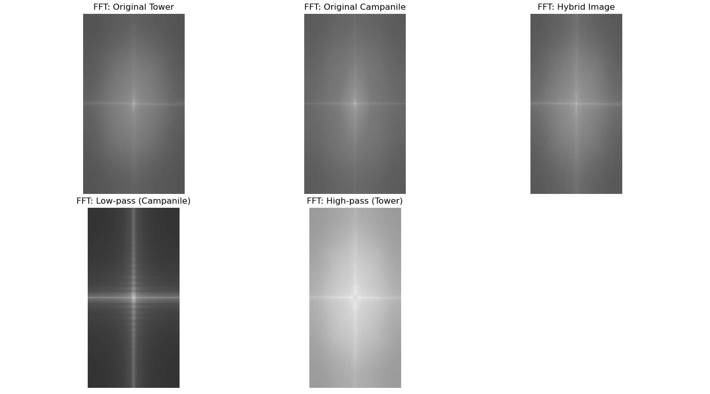
Part 2.2: Hybrid Images
Then in this next part, we combine the low frequencies of one image with the high frequencies of another image to get a hybrid image effect. Aside from testing it out on Derek and Nutmeg, I tried to create a hybrid between an Eiffel-looking tower and the Campanile. For the tower hybrid, I used a low-pass cutoff of 15 and high pass cutoff of 25.
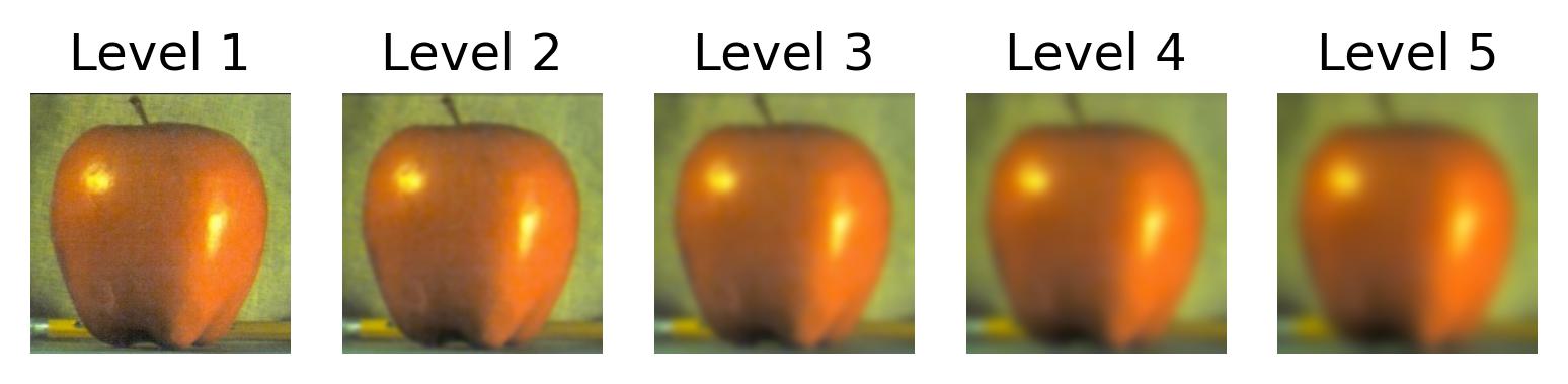
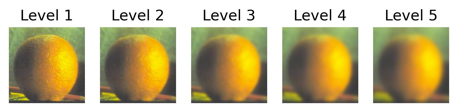
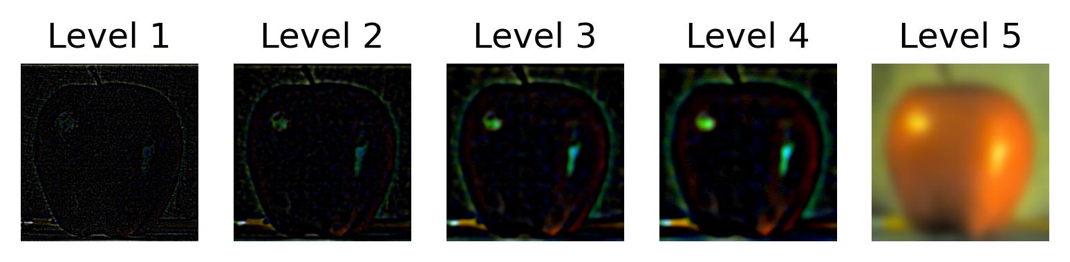
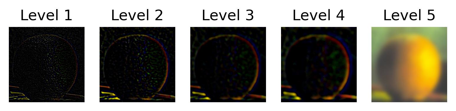
Part 2.3: Gaussian and Laplacian Stacks
This part uses Gaussian and Laplacian stacks to prepare us for the next part where we attempt to combine two images seamlessly. Here are the stacks on the provided apple and orange images.
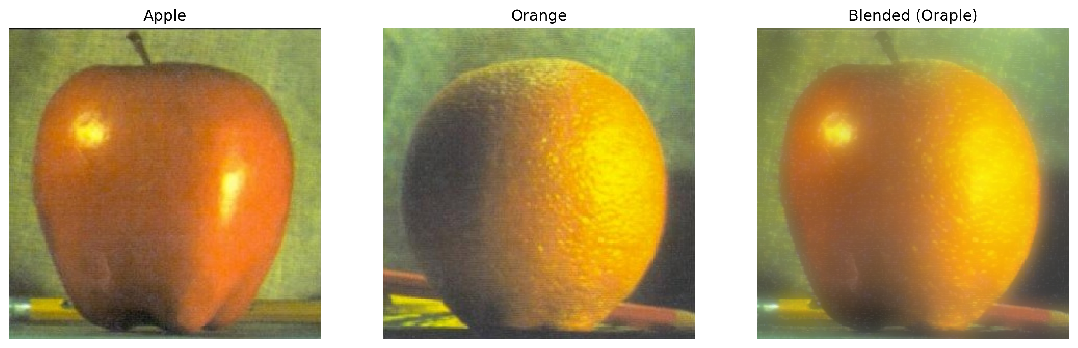
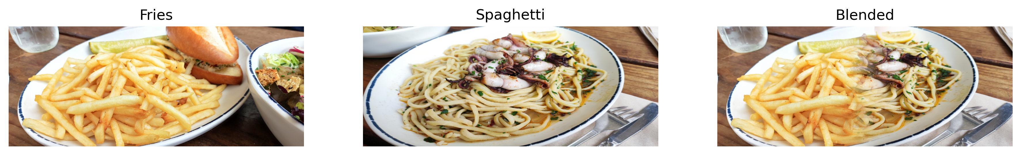
Part 2.4: Multiresolution Blending (aka. Oraple)
And finally we can visualize the oraple result as well as some other fun blends!