Part A.1: Projective Transforms
In this project, we use warping and detection techniques to "combine" separate images into seamless mosaics. First, we gather a few photos where we fix the center of projection and rotate the camera (also known as projective / perspective trasforms).
Part A.2: Recovering Homographies
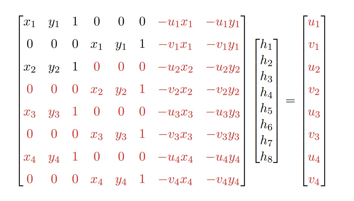
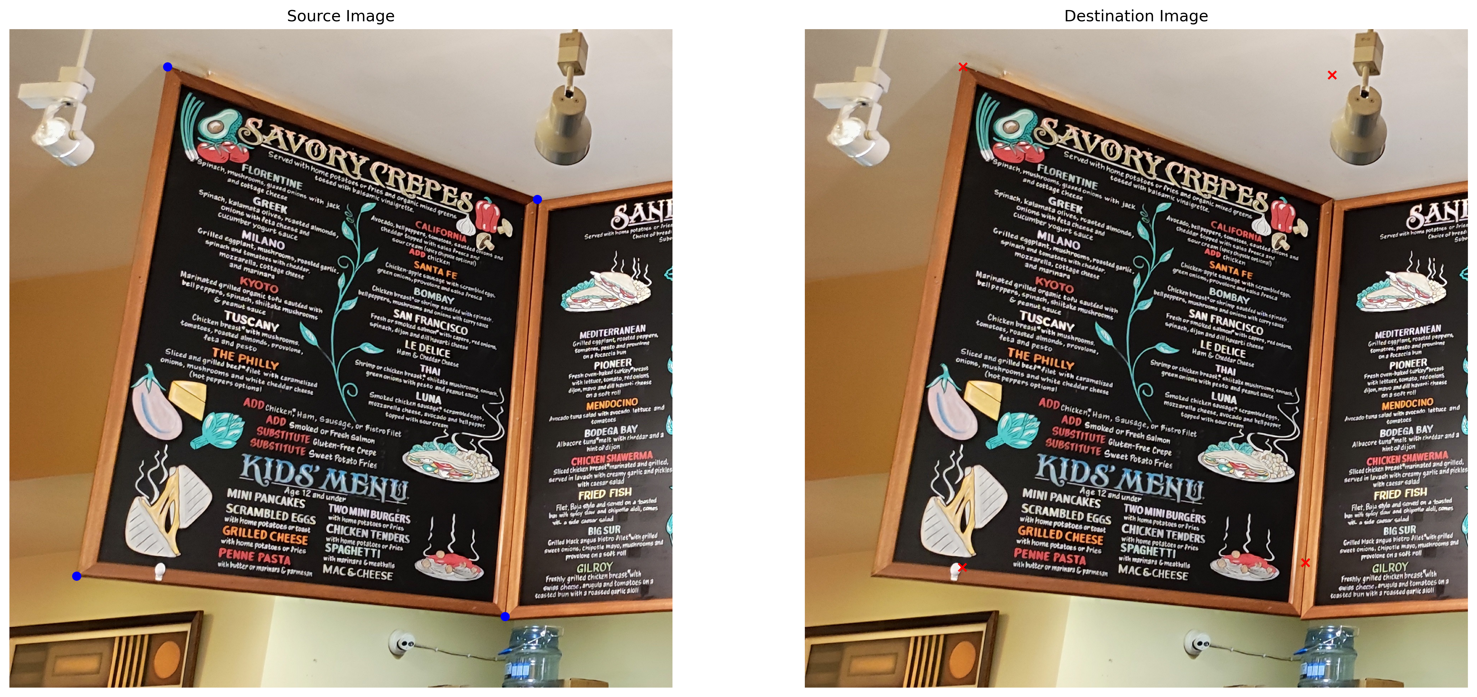
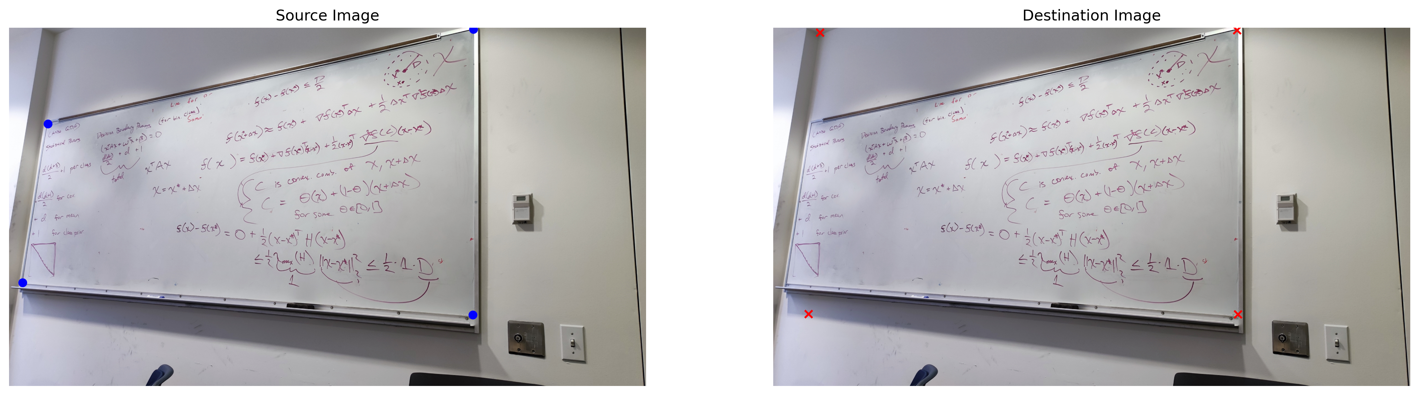
Next, we select correspondence points for our images so that we can compute a homography matrix that allows us to establish a mathematical relationship beteween the projective images.
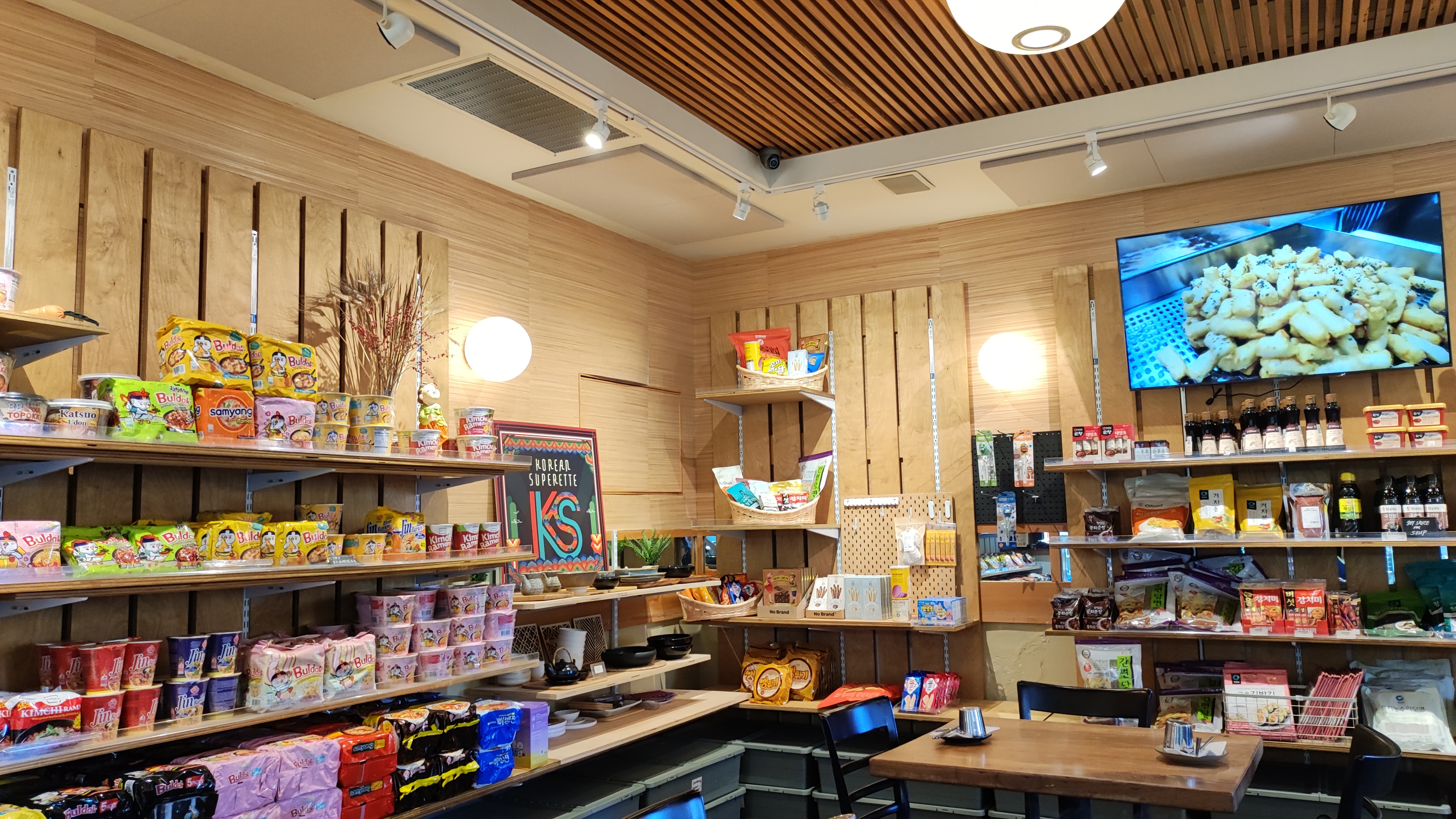
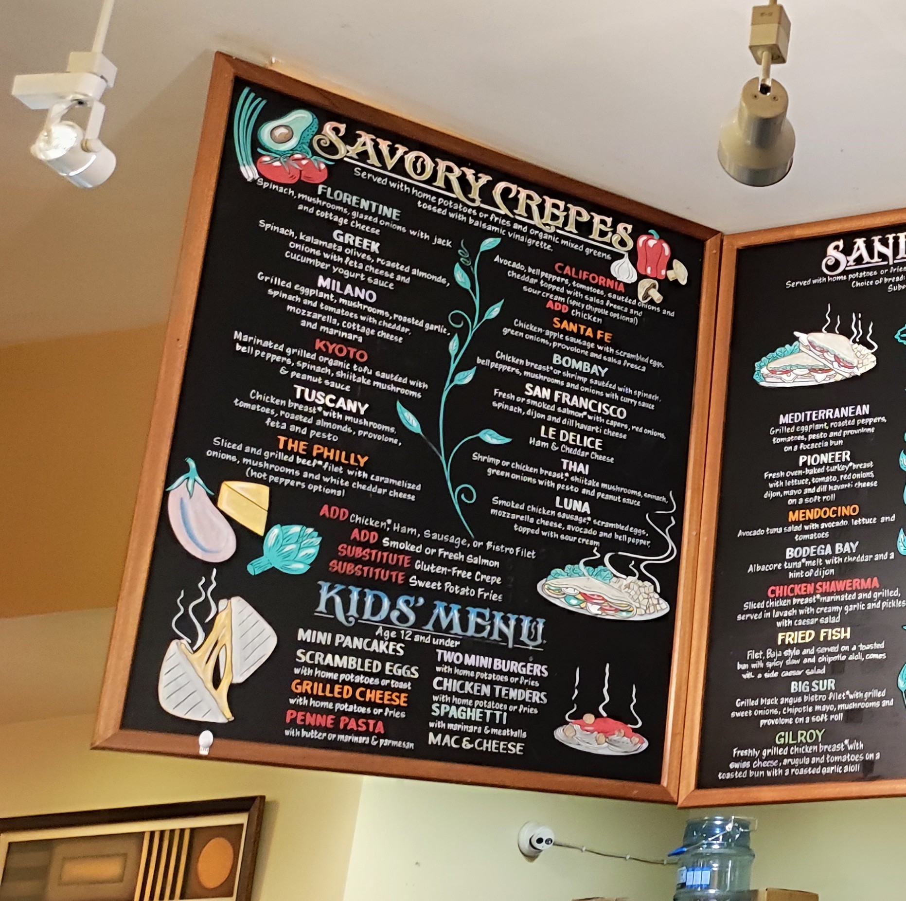
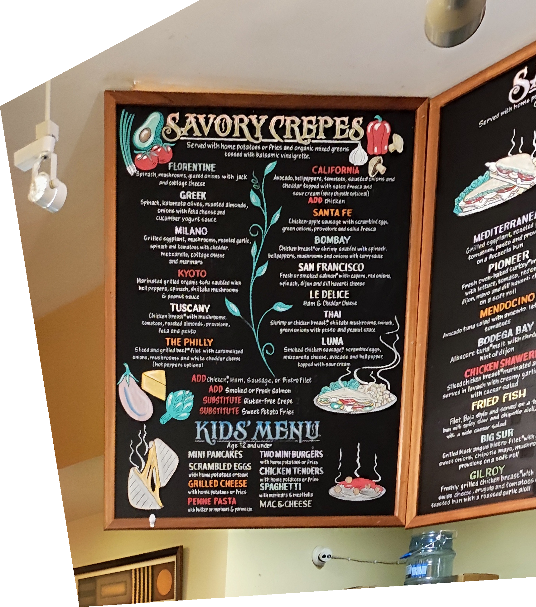
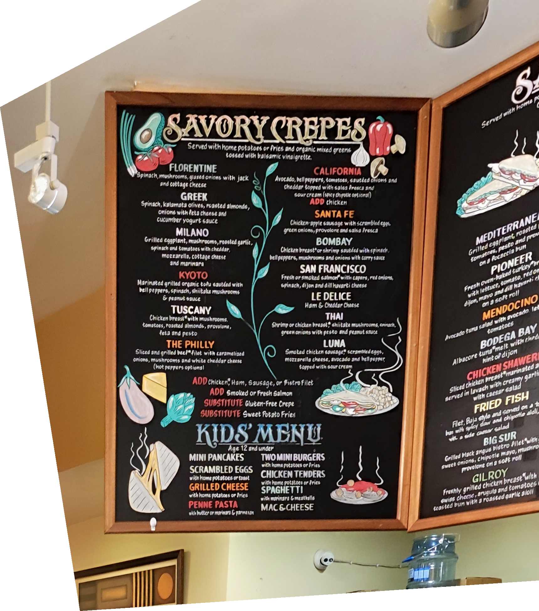
For example, this is the recovered homography matrix on the following menu board photo:
           [ 6.41627275e-01,  1.78404625e-01,  1.07327821e+02],
           [-3.80550278e-01,  1.06400977e+00,  1.54645094e+02],
           [-1.89449115e-04,  1.11919643e-04,  1.00000000e+00]
Part A.3: Image Warping
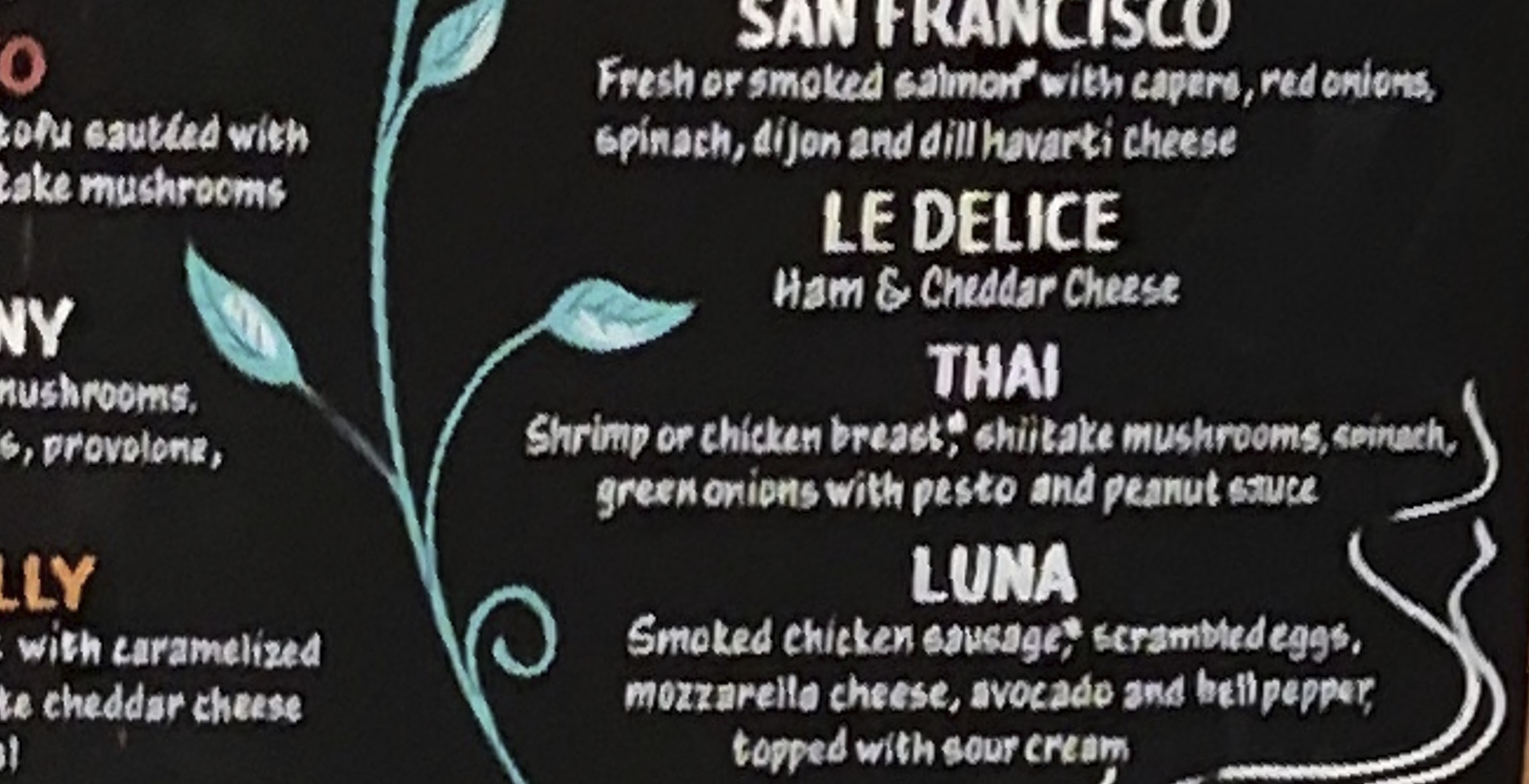
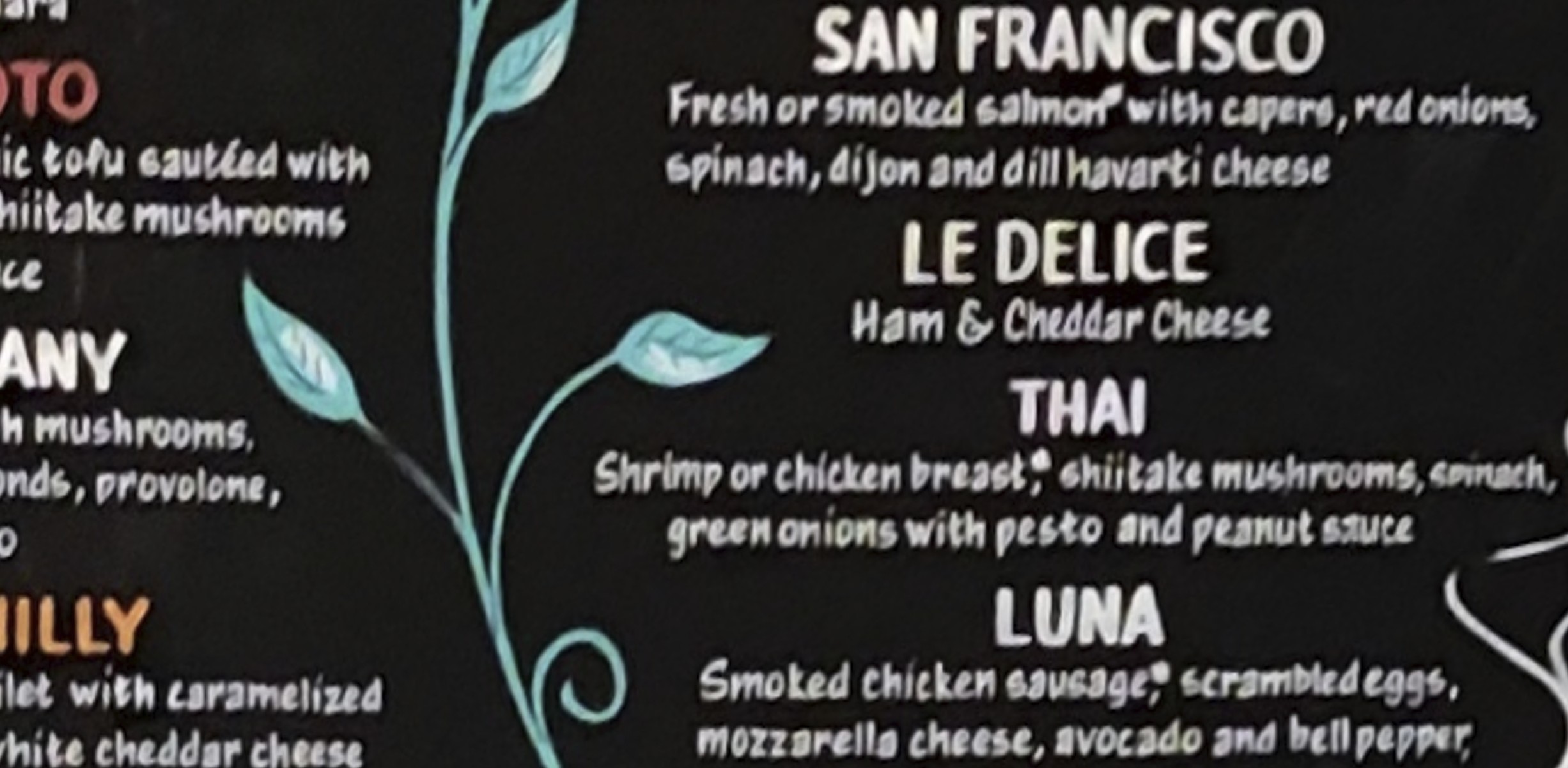
After recovering the homorgraphy matrix, we implement warping functions to warp our images. We try two different warping approaches here:
(1) Nearest neighbors: take the value of the nearest pixel
(2) Bilinear interpolation: take the average value of the nearest 4 pixels
As one can see from the rectified image details (may need to zoom in), bilinear interpolation produced smoother edges whereas the nearest neighbors approach produced jagged edges.

Part A.4: Mosaics
Finally, we use all of the components from the previous subparts to assemble our images into mosaics!
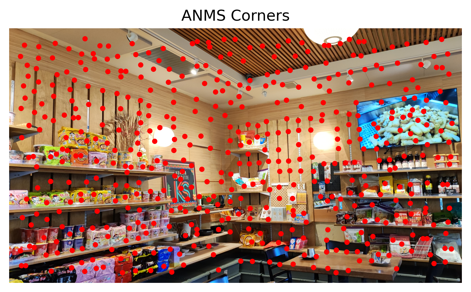
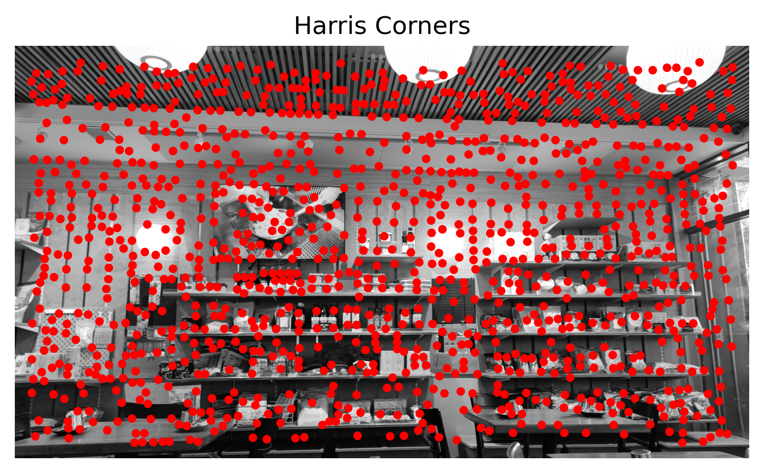
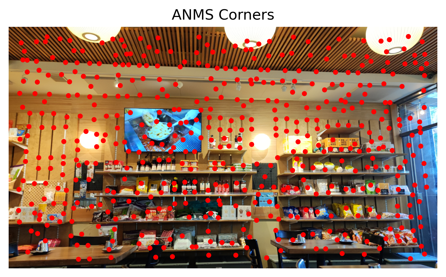
Part B.1: Harris Corner Detection
In part B, we try to "automate" the process we carried out in part A by using various techniques (corner detection, feature extraction, patch matching, RANSAC). First, we use Harris corner detection to gather coordinates that may serve as good coorespondence points. We focus on corners in particular because they have the most change in both x and y directions, making those parts of the image more distinguishable from other parts of the image such as a blank sky. After Harris corner detection, we use Adaptive Non-Maximal Suppression (ANMS) to reduce the amount of candidate coordinates.
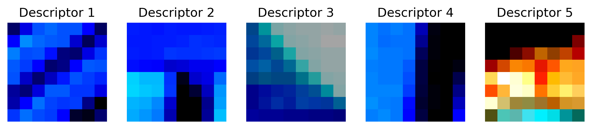
Part B.2: Feature Descriptor Extraction
With these coordinates, we can extract certain parts (patches) of the photos, which is known as feature extraction, such as the examples below.
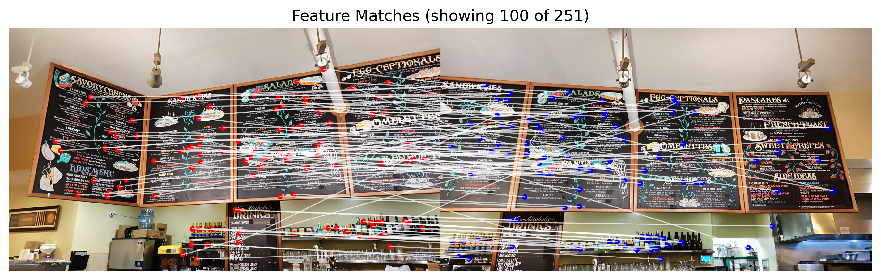
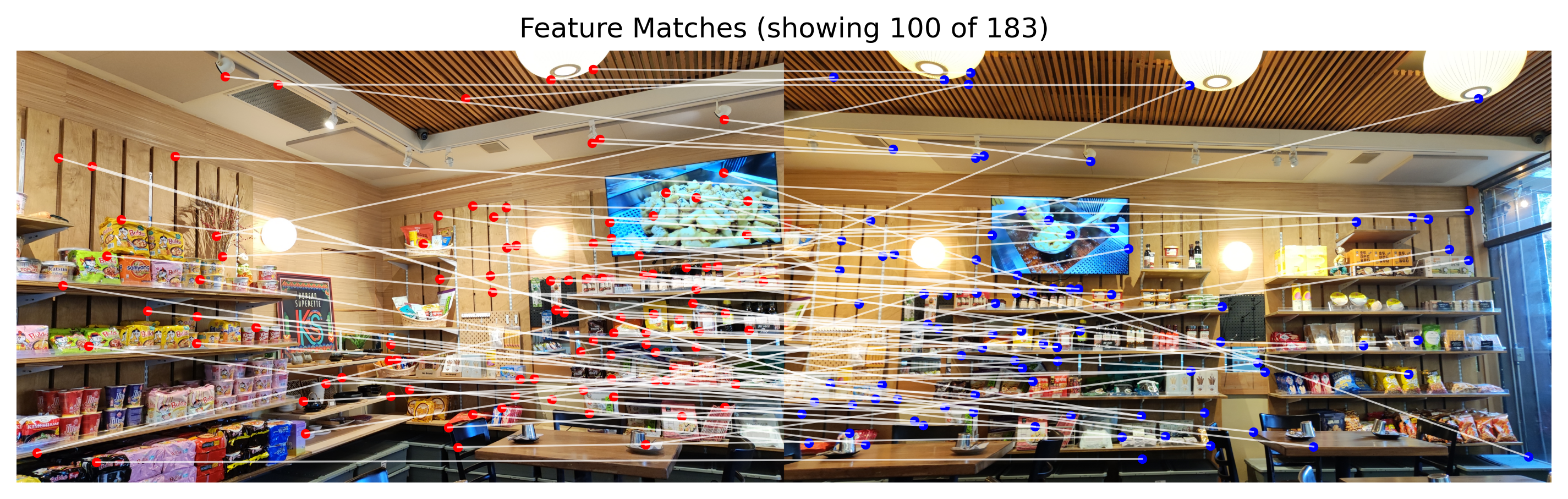
Part B.3: Feature Matching
Using feature patches in the left image, we attempt to recover their corresponding location (coordinate) in the right image to match the image parts together and develop a correspondence.
Part B.4: RANSAC
Finally, we run RANSAC to determine which of these correspondences are reliable or not and recompute our homography to yield better results. This allows us to constuct a mosaic.