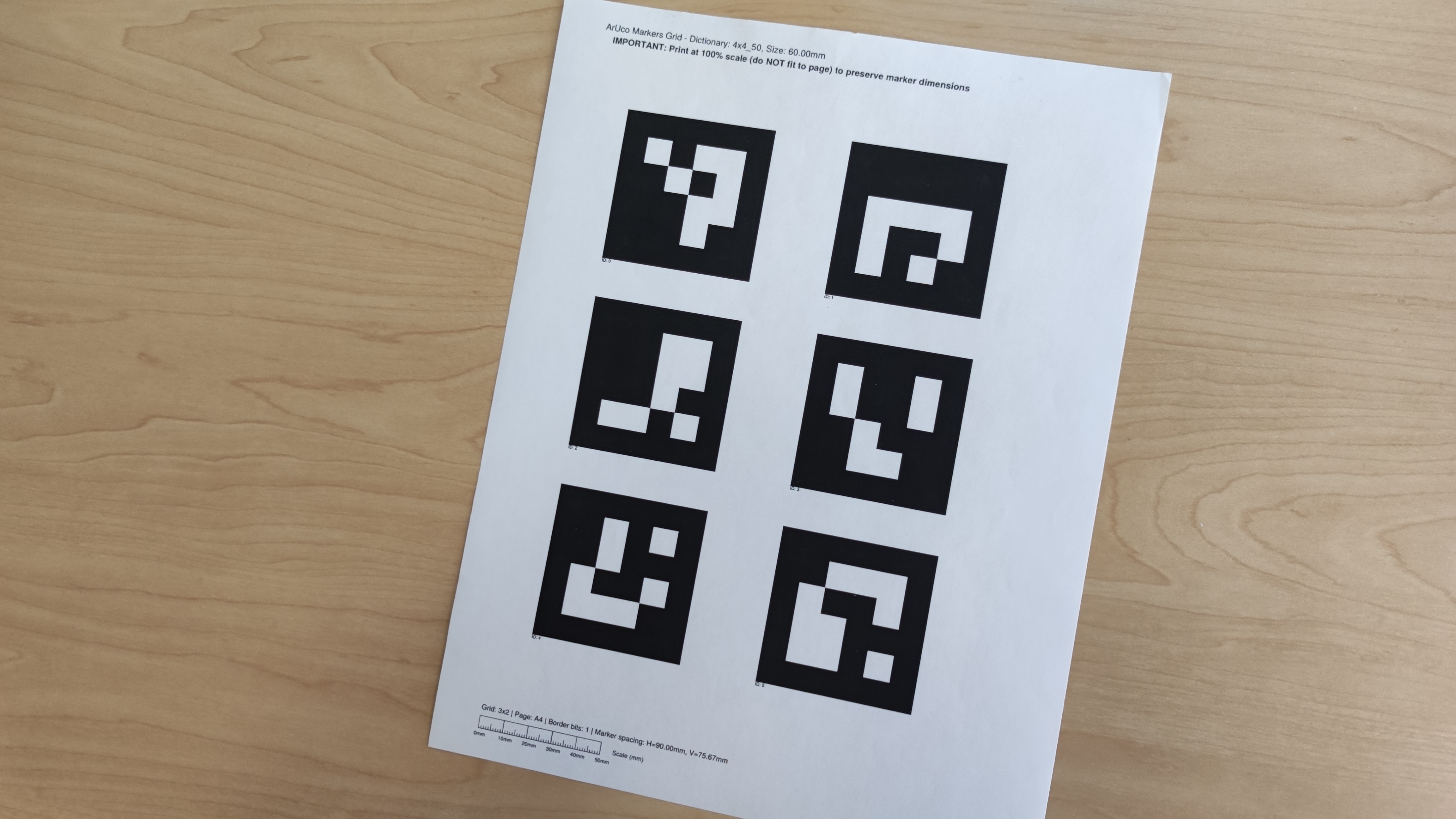
Parts 0.1 & 0.2: Camera Calibration & Capturing a 3D Scan
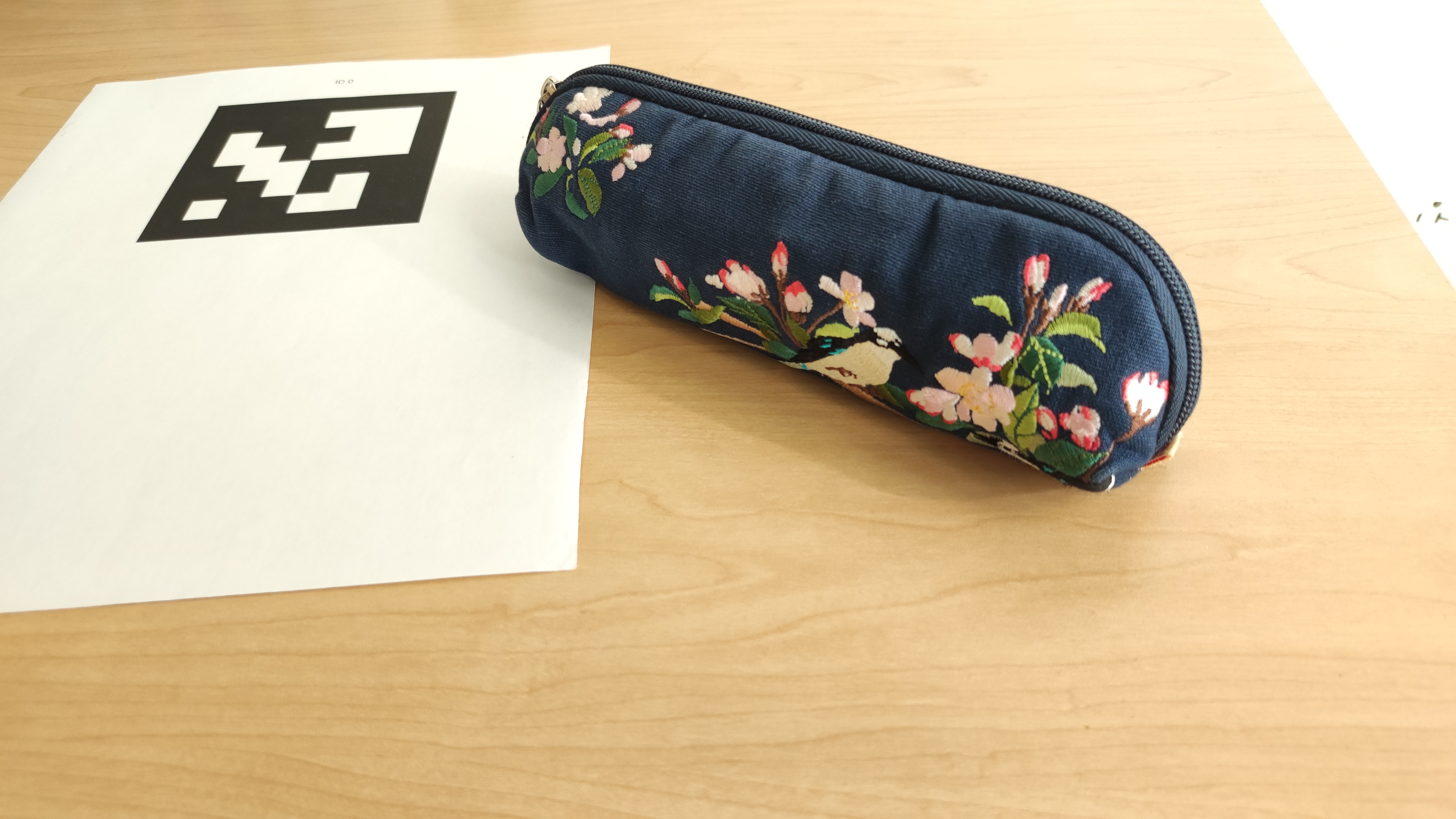
Before building the NeRF, we first print out a sheet of Aruco tags and take ~30 images of it from varying angles and distances while ensuring that the zoom is preserved. This allows us to calibrate our cameras with the help of cv2.calibrateCamera() and gather instrinsic parameters which are later used to estimate our camera pose. Afterwards, we captured a 3D scan of an object by placing it next to a single printed acruo tag and again taking ~30 images from varying angles and distances. I chose a pencil pouch as my choice of object.
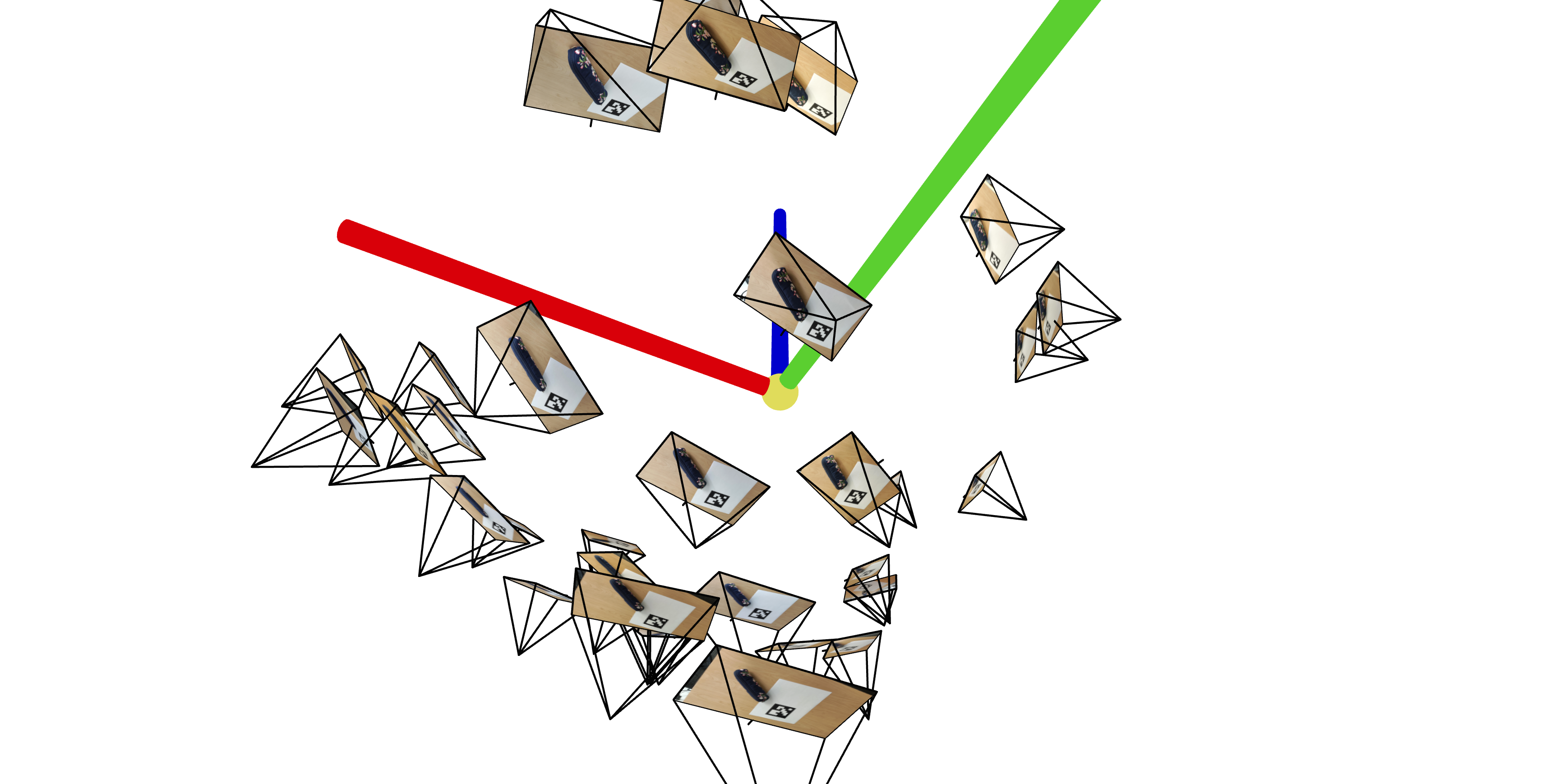
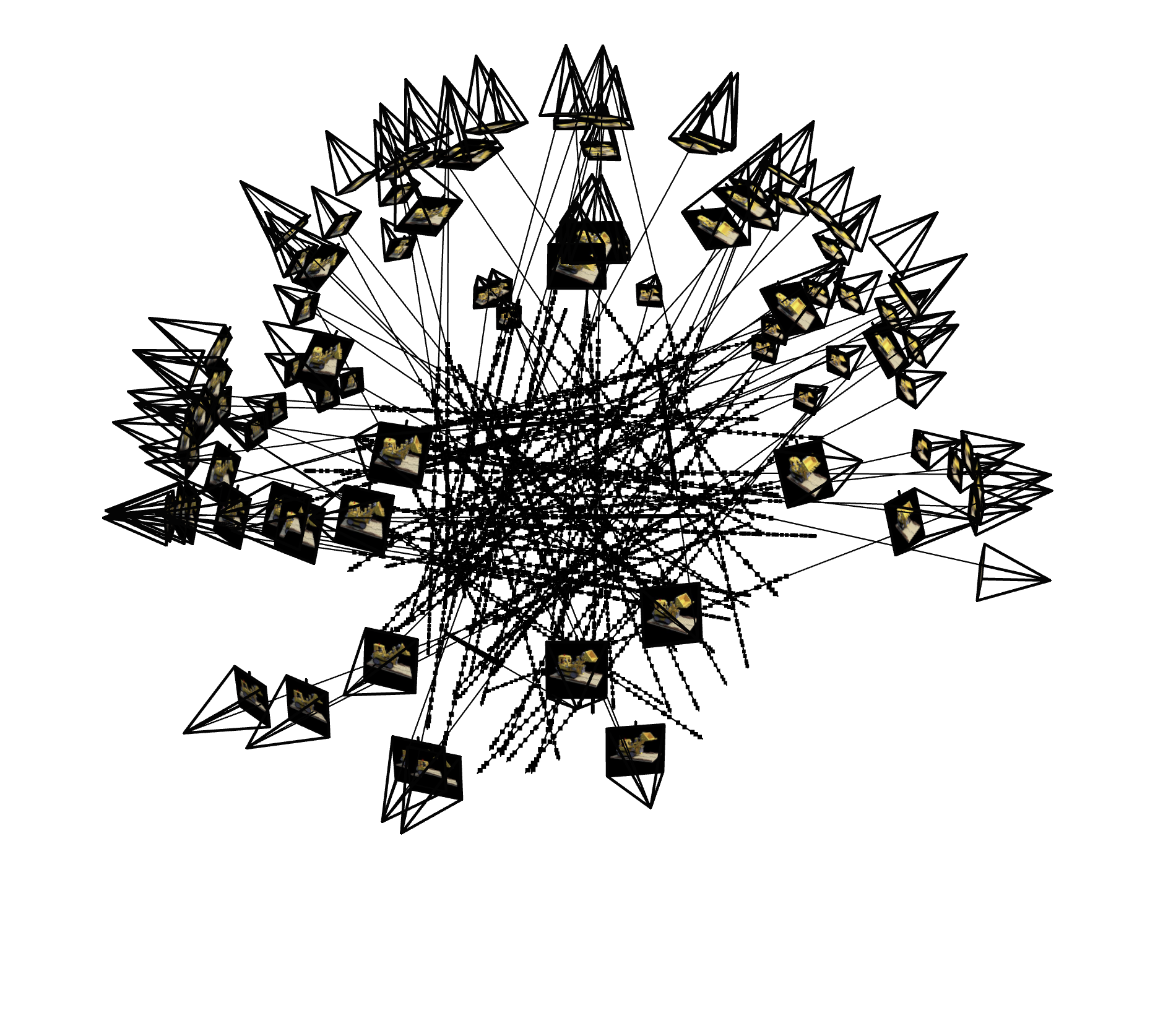
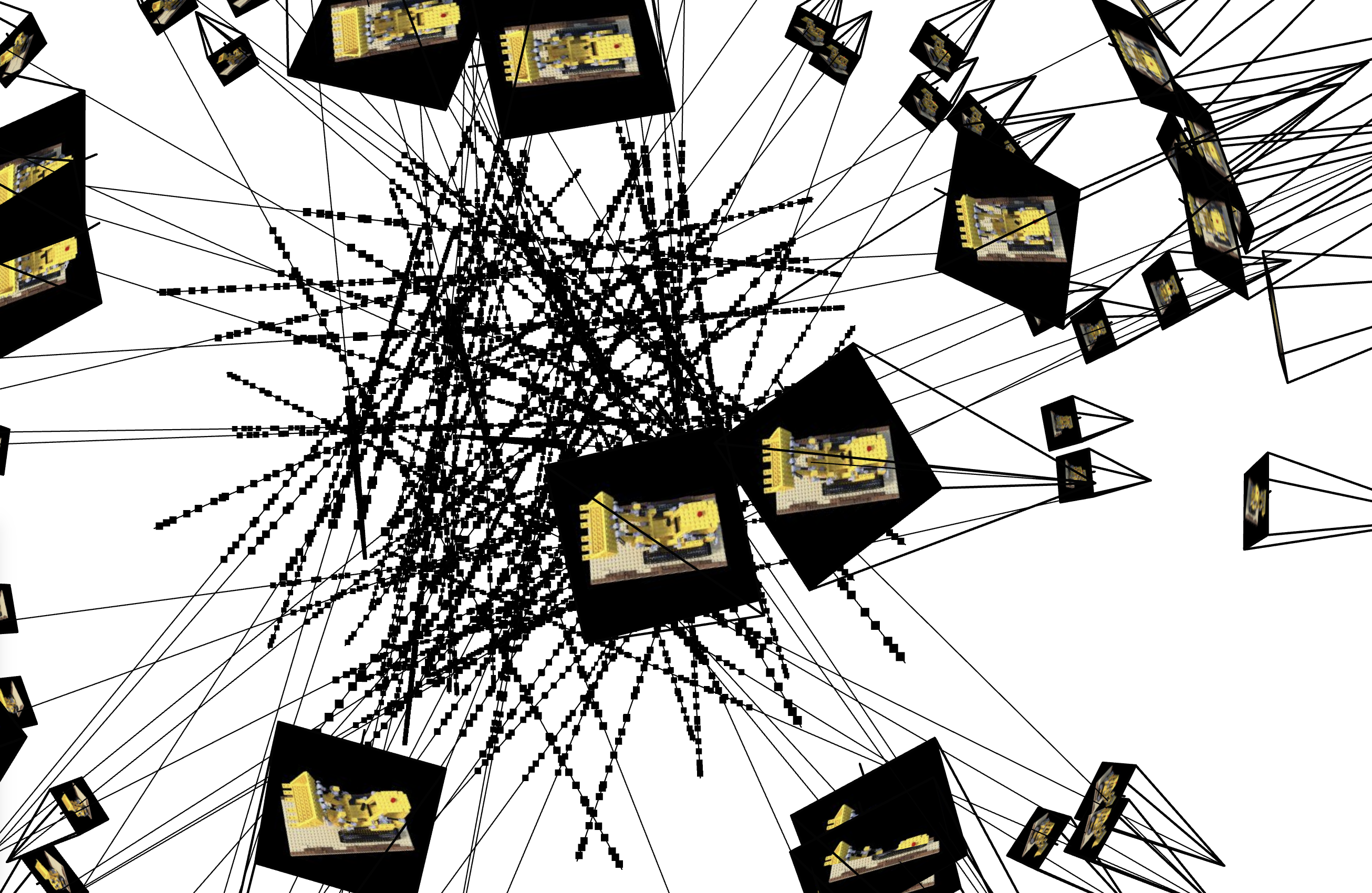
Part 0.3: Estimating Camera Pose
Using the camera calibration parameters from part 0.1, we estimate our camera pose by leveraging the rotation matrix and translation vector of our camera's extrinsic matrix along with cv2.solvePnP (and of course, linear algebra). We then pass these into a visualization tool, viser, to observe the poses in 3D space. Here are the 3D visualizations of my pencil pouch scan:

Part 0.4: Undistorting Images & Creating a Dataset
To wrap up part 0, we remove lens distortions from our images and organize everything into a dataset so that we can use it for NeRF training later on. We also split the data into training, validation, and test sets.
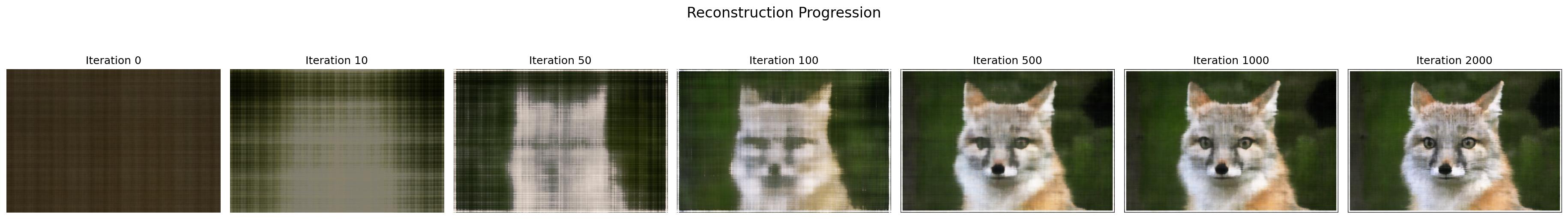
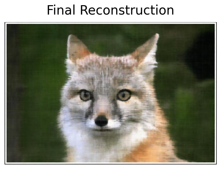
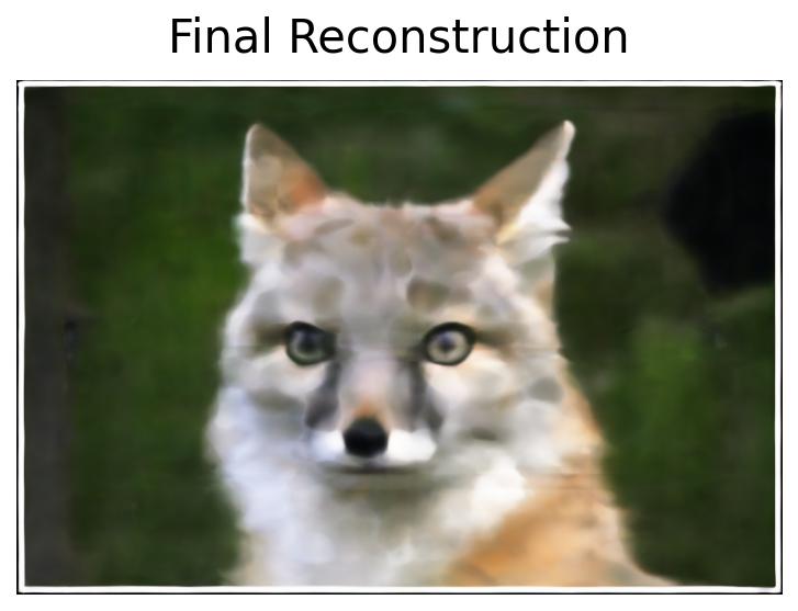
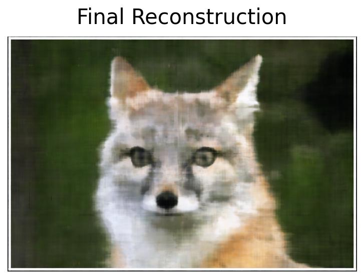
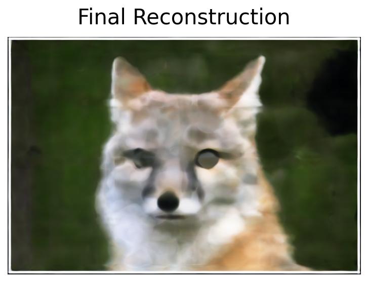
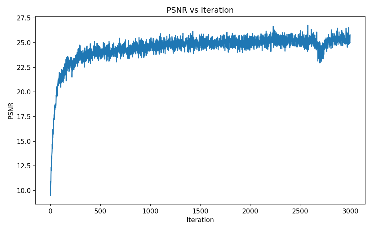
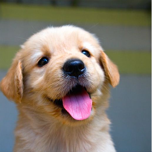
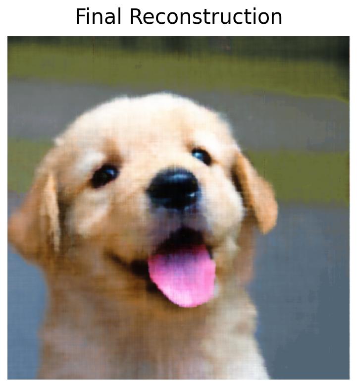
Part 1: Fitting a Neural Field to a 2D Image
To prepare us for 3D NeRF work, we first focus on 2D Neural Fields. Namely, we build a multilayer perceptron (MLP) that when given an image, attempts to reconstruct it by using pixel coordinates as inputs and outputting some rgb color value. The architecture of my model closely followed the one that is provided in the project specifications (4 Linear layers with ReLUs in between, width of 256, learning rate of 1e-2, Adam optimization, MSE loss).
Part 2.1: Creating Rays
After playing with 2D MLPs, we move on to 3D first by implementing a few functions that help us convert between coordinates.
1. Camera to World Coordinate conversion
2. Pixel to Camera Coordinate conversion
3. Pixel to Ray conversion
In a nutshell, (3) uses (1) and (2) to tranform from pixel to camera, and camera to world to locate ray origin and direction.
Part 2.2: Sampling
Then, we develop a few sampling functions to collect samples along rays.
1. Sampling Rays from Images
2. Sampling Points along Rays
(1) randomly samples rays from a batch of images. For each image, it computes the ray origins and directions (with (3) from 2.1) by leveraging a meshgrid of randomly chosen pixel coordinates. The corresponding RGB values are gathered from the image at those pixel locations and combined along with rays to train our model later on. (2) uses near and far bounds (of 2 and 6) to create evenly spaced depths. It also allows for random perturbation of sample points to allow for better variation in our sample.
Part 2.3: Dataloading
Afterwards, we create a 3D dataloader just like we did in part 1 for the 2D MLP which enables us to compute ray origin, ray direction and pixel colors using the previous subparts. Here are a few visualizations of the samples with the help of viser:
Part 2.4: Neural Radiance Field
In this part we finally build the NeRF structure! It uses a comparable structure to the one in part 1, but with a few key modifications First, the input now takes in 3D world coordinates and outputs the density along with the color. Additionally, the MLP structure is deeper (still Linear and ReLU layers) and includes skip connections as well as branching: one for density, one for rgb / color. The concatenation (skip connection) occurs in two places, one for the density branch, and one for the color branch. And it still uses Adam / MSE loss but now with a learning rate of 5e-4.
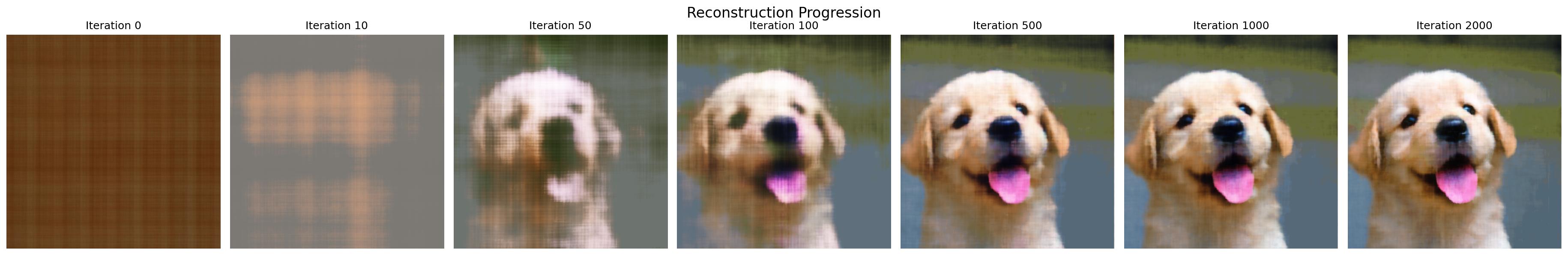
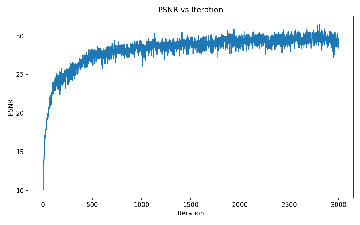
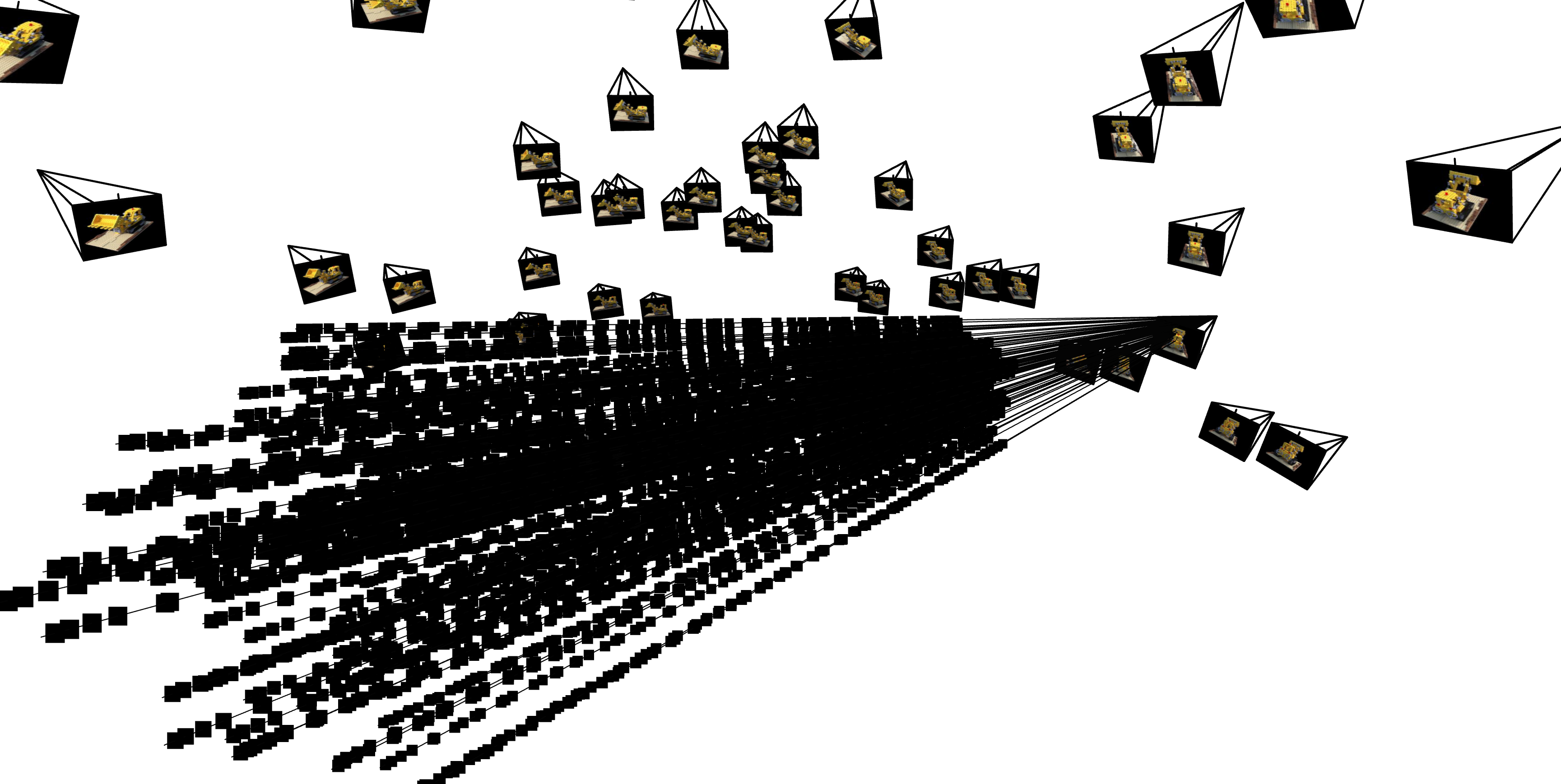
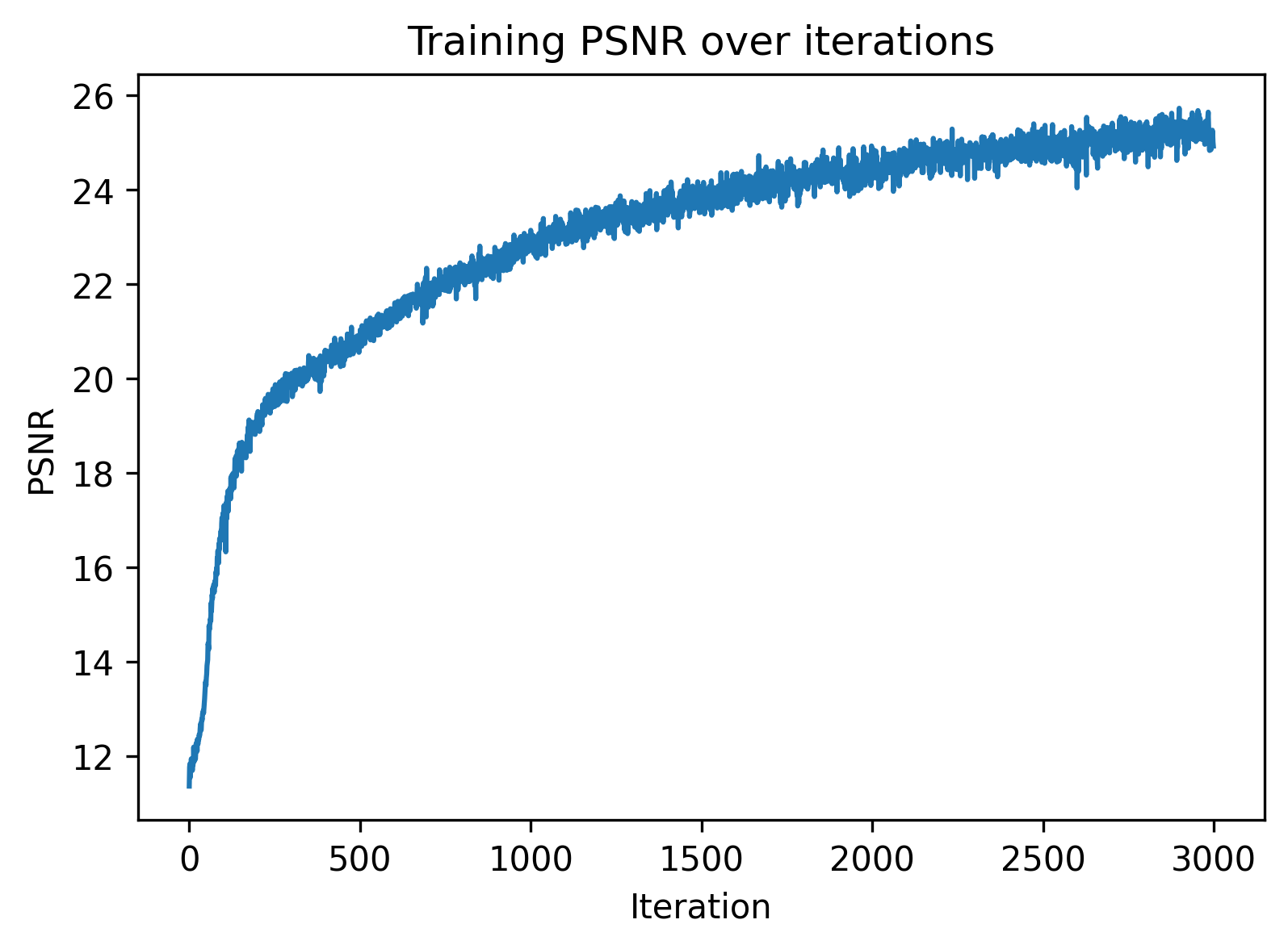
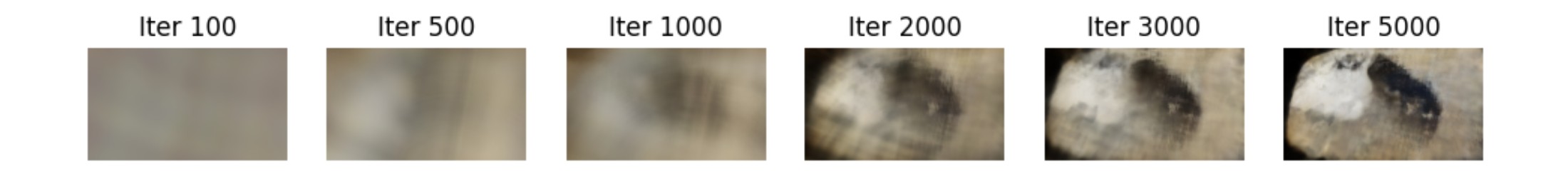
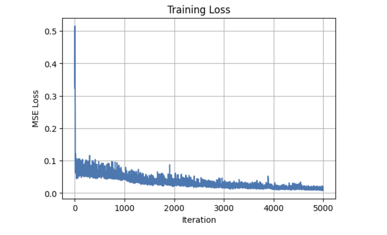
Part 2.5: Volume Rendering
We then build a volume rendering function that converts densities into alpha (absorption) values and combines it with transmittance to predict colors. After doing so, we have all the necessary components to train our NeRF model. Here we visualize the training process on the provided lego dataset.


Part 2.6: Training with Own Data
Finally we combine the previous parts and train a NeRF on our data from part 0 (my pencil pouch!).

And we're done (with arguably one of the hardest projects I've ever worked on)!