Part A.0: Setup & Text Prompts
In part A of the project, we experiment with diffusion models, sampling loops, and use them for tasks such as inpainting and creating optical illusions.
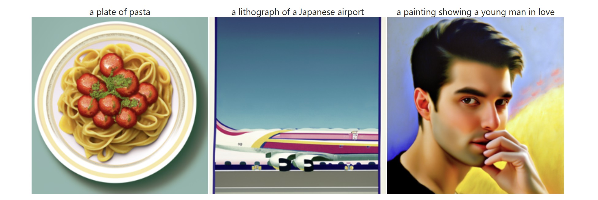
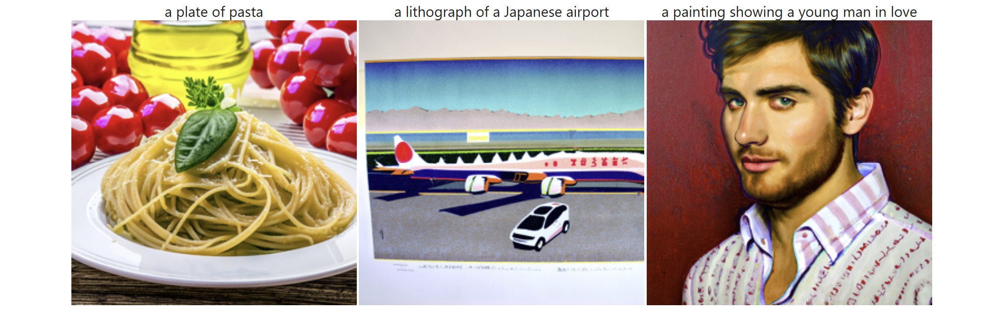
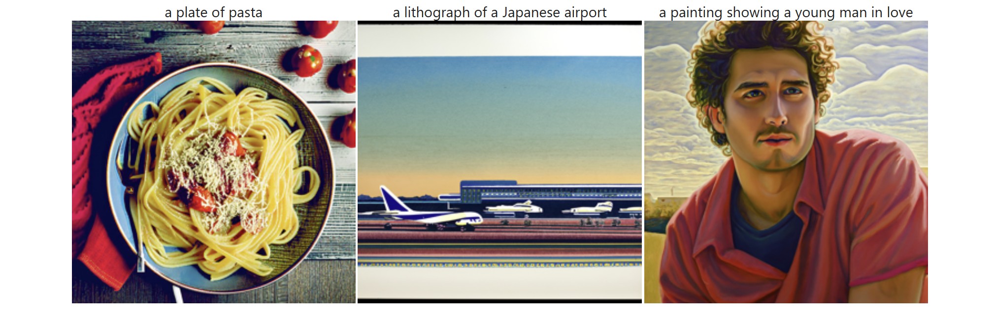
First, we obtain access to the DeepFloyd model and generate our own text prompts which we use to create images. I ran the model using a random seed value of 180 and tried out several different combinations for num_inference_steps using 20 and 200. At num_inference_steps = 20, the outputs were decent but not impressive. It was somewhat obvious that the outputs were AI-generated as they didn't look very realistic (especially due to the colors) and didn't have much texture / detail. Meanwhile, at a value of 200, the outputs had much more detail but the colors still looked somewhat exagerrated, especially for the pasta prompt. For the airport prompt, I think it could have done a better job making it clear that it was an airport in Japan specifically, and for the "man in love" prompt, I think it wasn't super obvious that the person was in love (except for maybe the first output with num_inference_steps = 20) -- it seemed like a normal glance and the expressions didn't look soft. I also tried a num_inference_step value of 400 and interestingly, there were visible small circles in the outputs.
A.1.1: Implementing the Forward Process
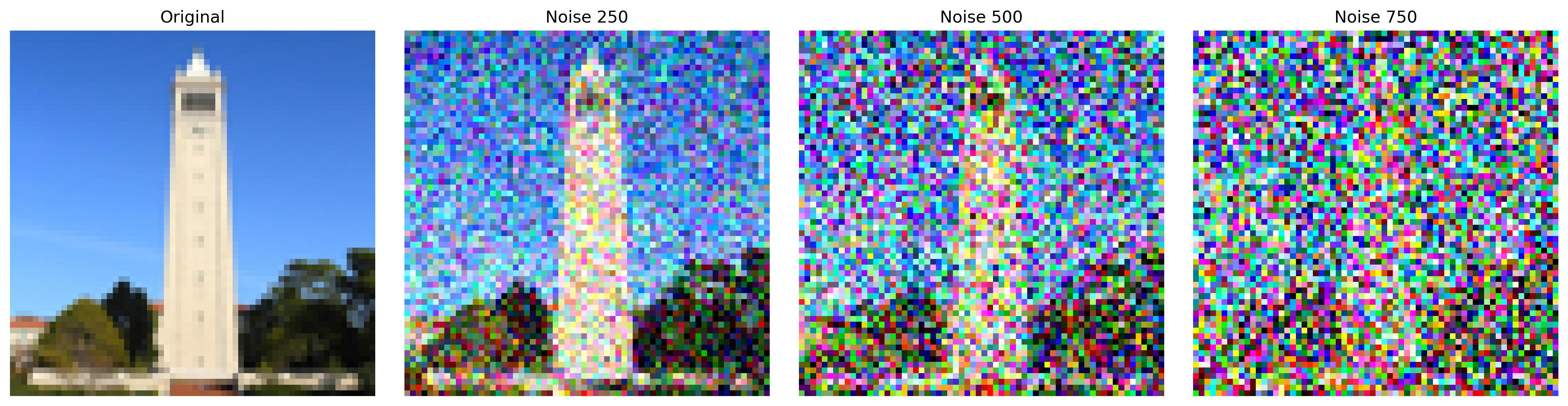
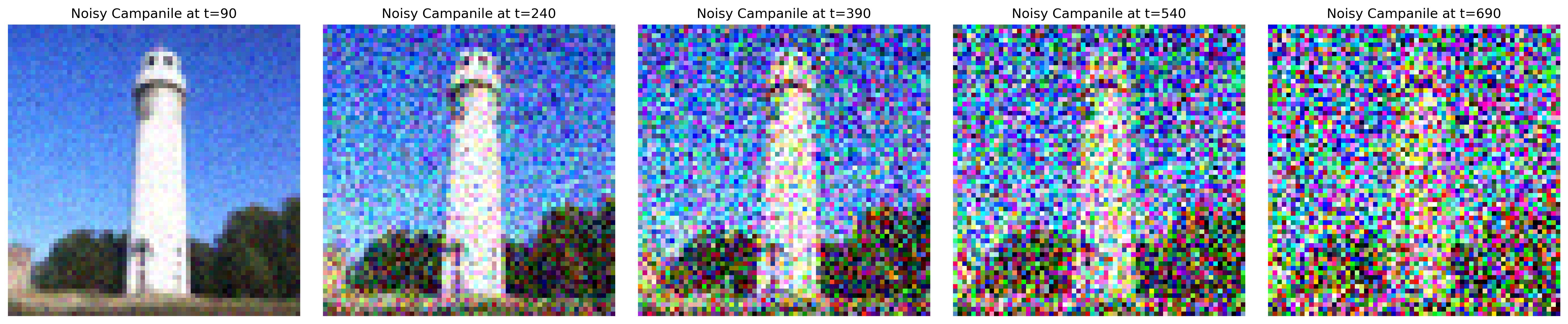
Next, we move on to sampling loops by making use of the pretrained DeepFloyd denoisers. In this first subpart, we prepare ourselves for denoising by iteratively adding noise to a clean image. That is, given a clean image, we sample from a Gaussian (using mean and variance), apply scaling, and get a noisy image at a particular timestep. This process is stored in a "forward" function, and here are the results on an image of the campanile:
A.1.2: Classical Denoising
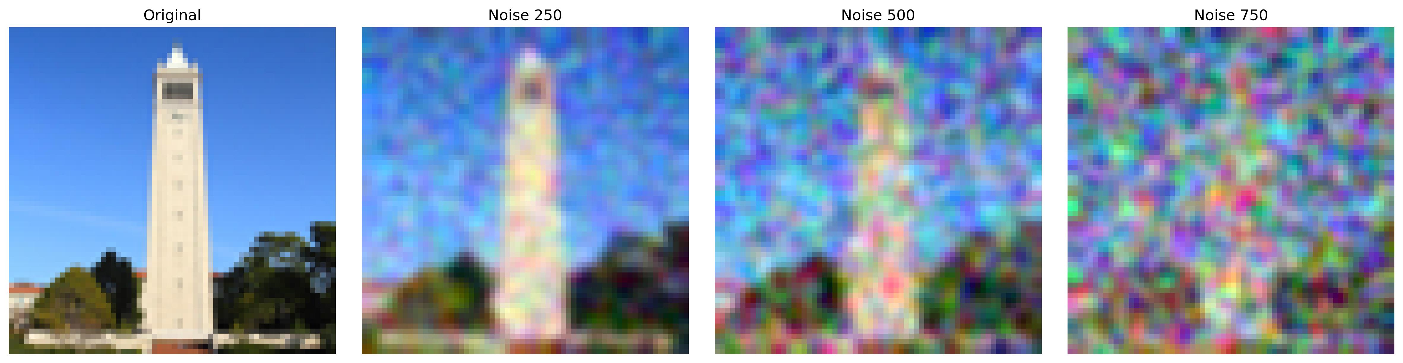
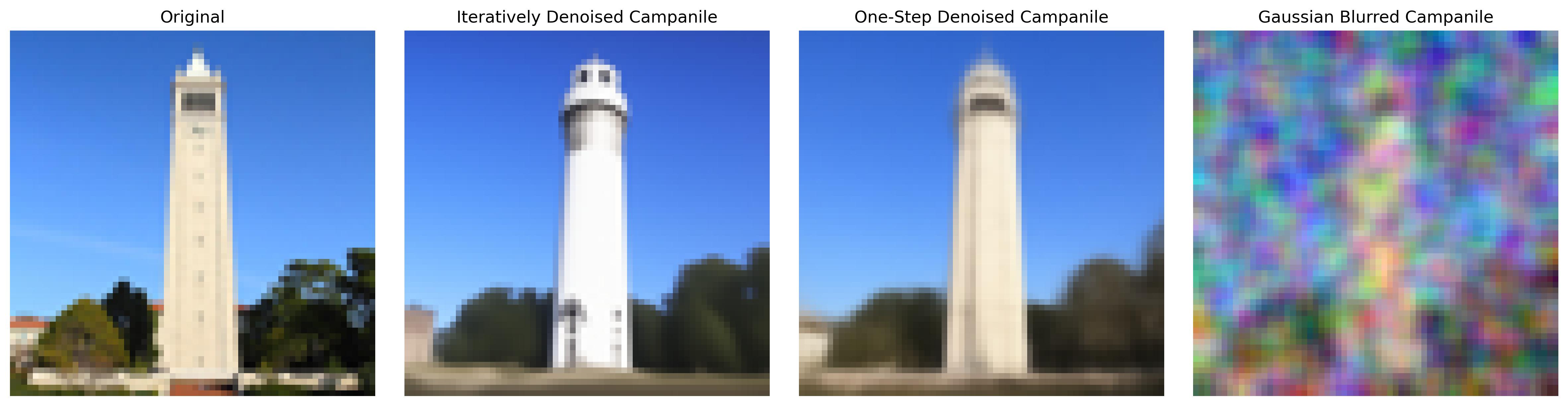
Next, we are ready for denoising. In classical denoising, we use Gaussian blur filtering to try to remove noise. After applying forward on our images, we use torchvision.transforms.functional.gaussian_blur to apply the gaussian blur filter. Here I used a kernel size of 5, and as we can see, the image looks smoother but the essence of the campanile remains destroyed:
A.1.3: One-Step Denoising
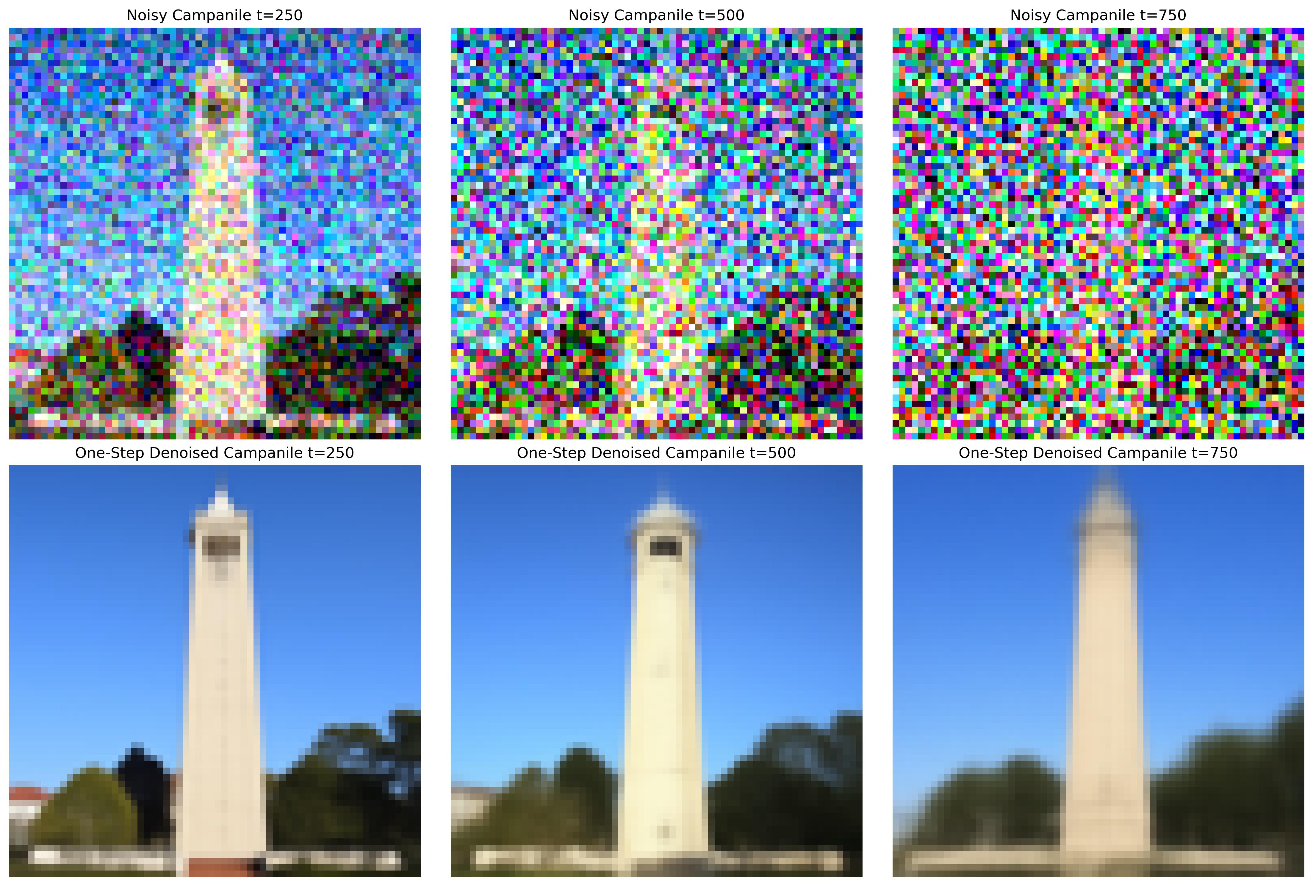
Then, we use a pretrained diffusion model (stage_1.unet) to denoise. Aside from applying forward to our campanile image, we estimate the noise in the new noisy image by passing it through stage_1.unet. Using this, we can then remove noise from the noisy image to obtain an estimate of the original (clean) image. Importantly, we don't remove the noisy directly; we must scale the noise before removing since the forward process adds a *scaled* version of the noise. The results do no disappoint:

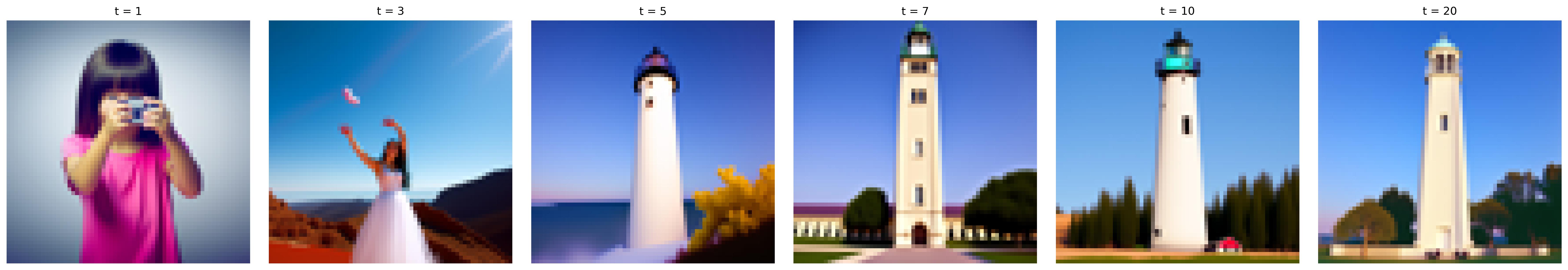
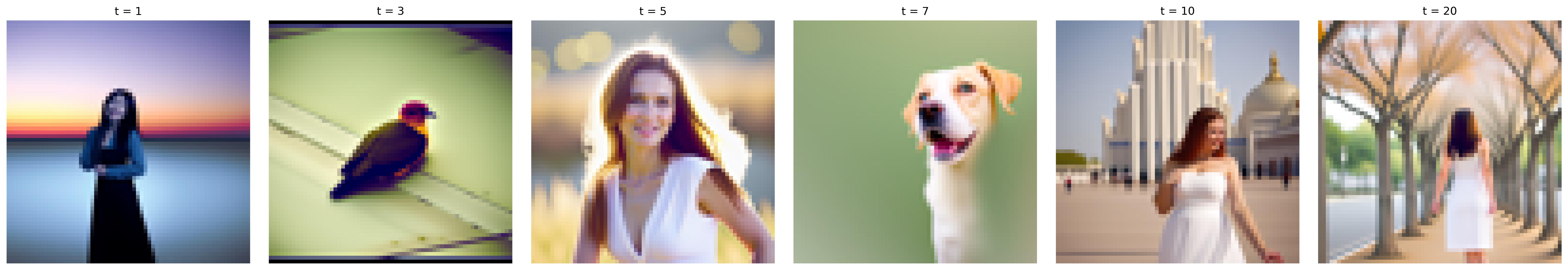
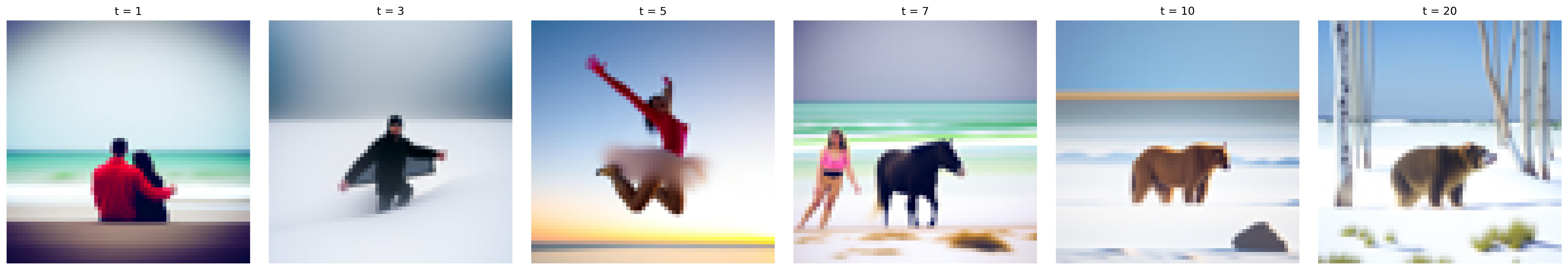
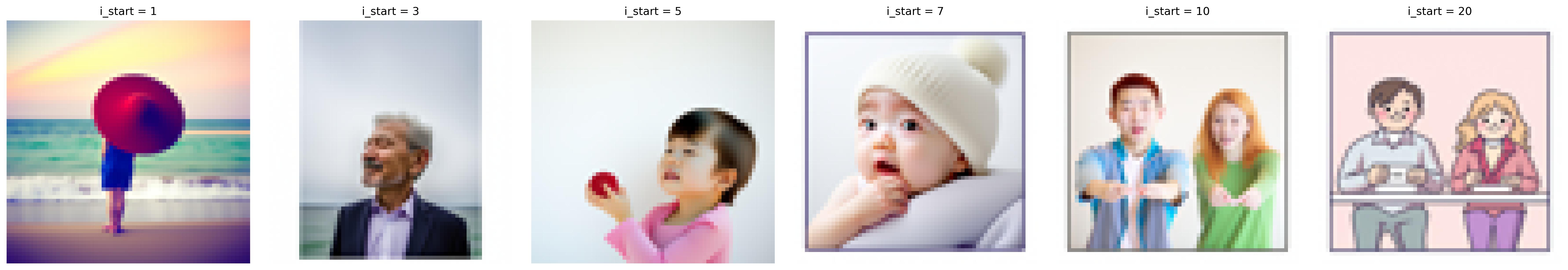
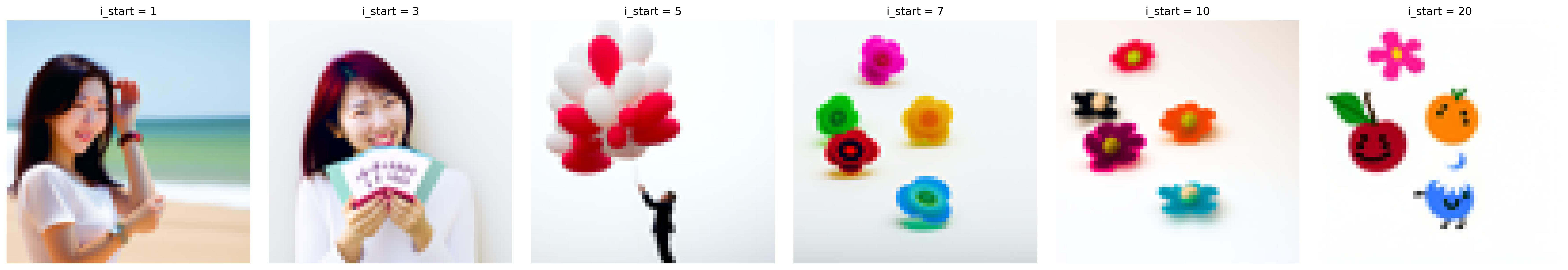
A.1.4: Iterative Denoising
Although 1.3 is great, we can see that the quality of the results deteriorate as the images become noisier. To address this, we try denoising in an iterative manner -- using timesteps. However, we do not want to go through all steps from 1 to n as that would be super slow, so we take our steps in strides of 30. This is done by creating a function that denoises our image at some starting timestep index (timestep[i_start]), applying a mathy formula to obtain an image at the next timestep (t' = timestep[i_start + 1]), and repeating the process until we produce a clean image. Here are some figures for comparison:
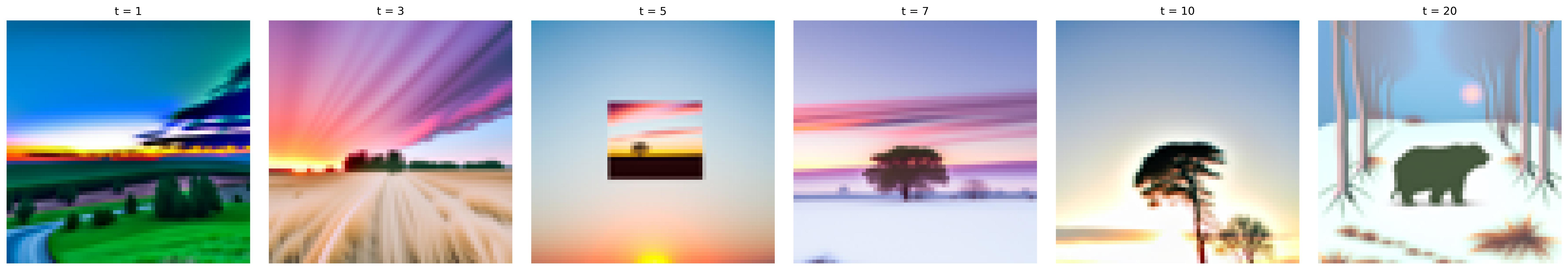
A.1.5: Diffusion Model Sampling
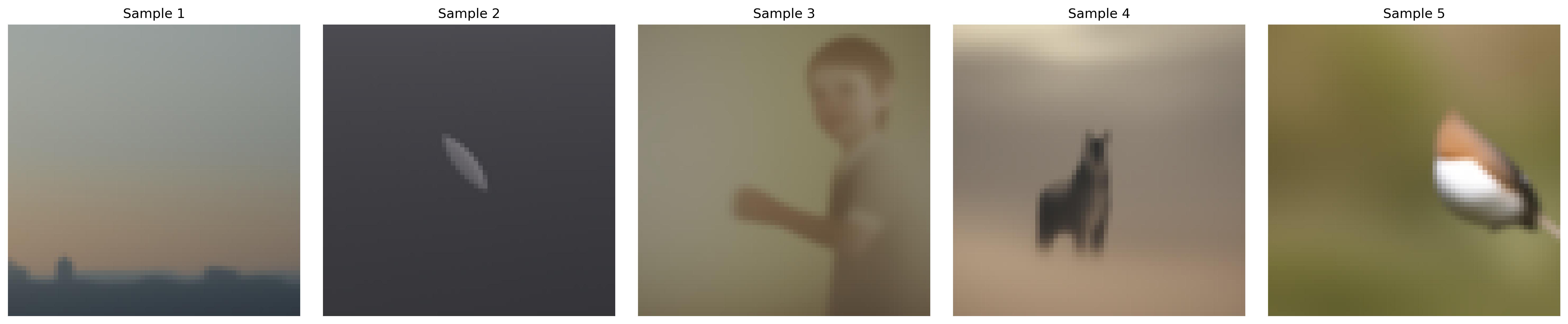
Aside from denoising images, we can also use the denoising model to generate images from scratch. This is done by setting our starting index / timestep as 0 and in our noisy image as random noise, which in effect denoises pure noise. To visualize the results, we take 5 samples of the prompt "a high quality photo".
A.1.6: Classifier-Free Guidance (CFG)
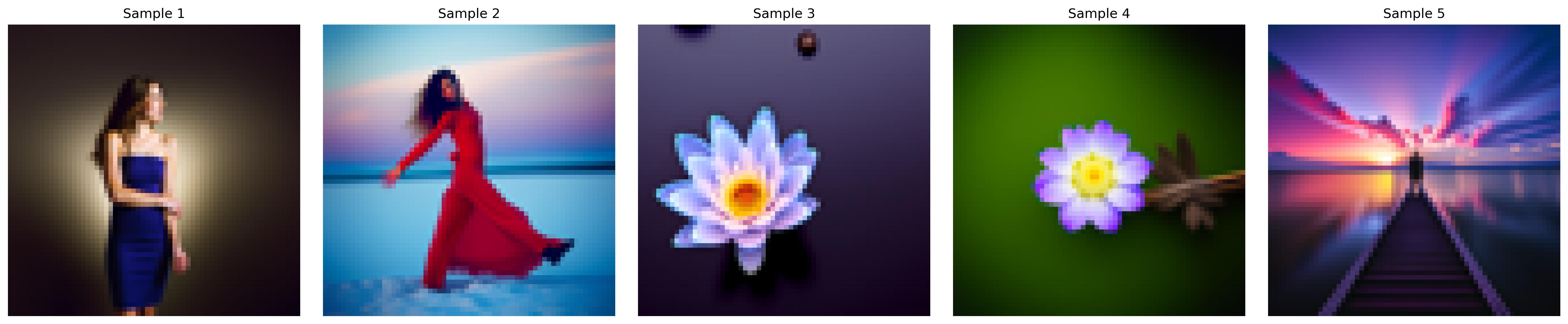
The results in 1.5 were not great, but we can improve this with CFGs! In CFG, we compute both a conditional and unconditional noise estimate then scale their difference and sum them up to "condense" them to a sinlge noise. Our scale controls the strength of the CFG (how closely we want our generated images to follow our text prompt). These are the results on the same "high quality photo" prompt using a scale value of 7. For all subsequent subparts, we use CFGs.
A.1.7: Image-to-image Translation
Now that we have CFGs, we can get a little more creative! Here, we generate an image that is similar to the campanile by applying a series of edits to a random nose-generated image. We then take the original campanile image, add a little bit of noise using forward, and run iterative_denoise_cfg from 1.6. This produces a series of edits to our random image, each step getting closer and closer to original campanile. We also try the process on some other images, producing really cool results!
1.7.1: Editing Hand-Drawn and Web Images
We can also apply the process on illustrations! Here are the edits made on web and hand drawn images.
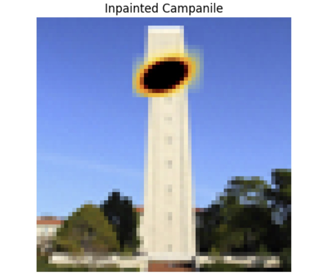
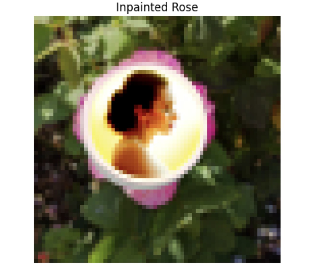
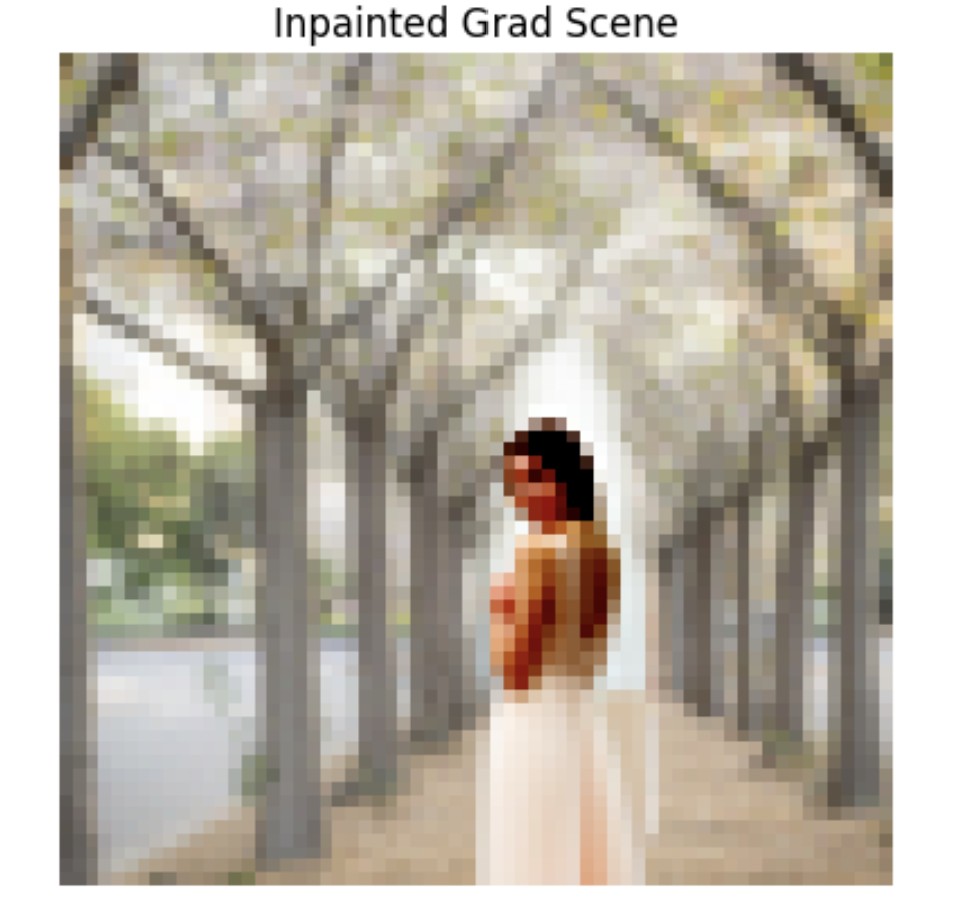
1.7.2: Inpainting
Another cool application of this is image inpainting. Here are the results on a few images (campanile, rose, grad photo scene from Berkeley's cherry blossom trees).
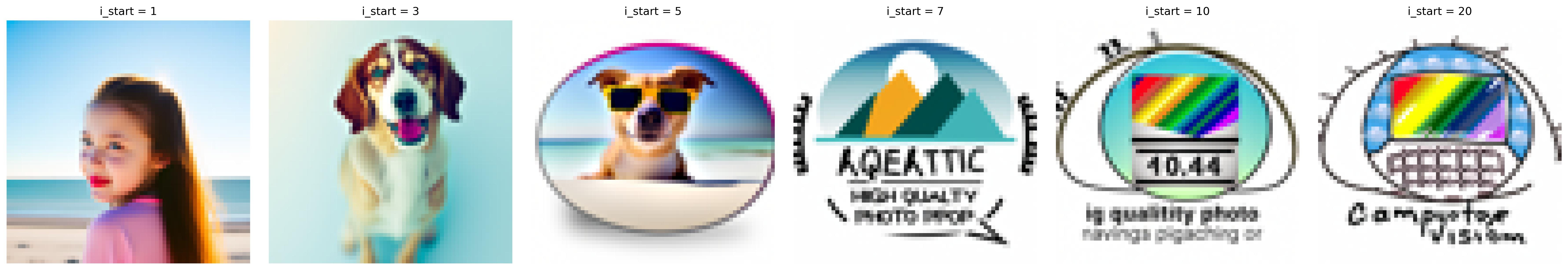
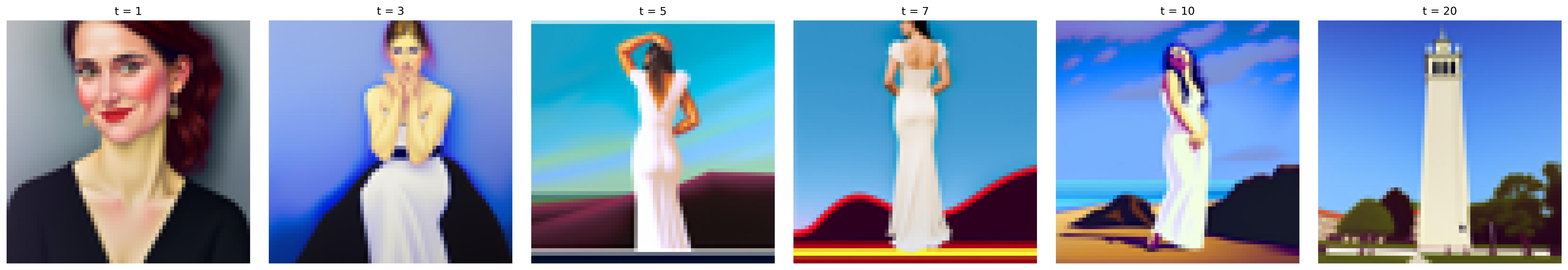
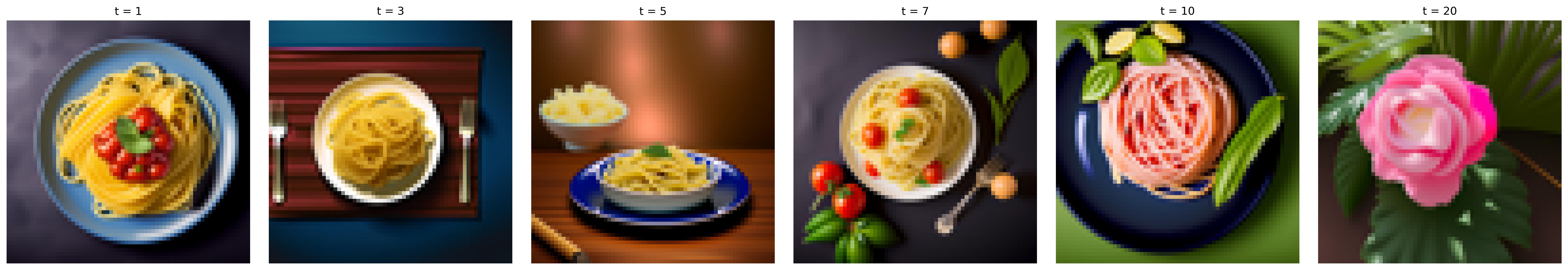
1.7.3: Text-Conditional Image-to-image Translation
Aside from passing in "a high quality photo" as our prompt, we can give our model a specific prompt, and as we can see, it will make edits on an image that matches our prompt instead of a random image. By doing so we are essentially guiding our model with a text prompt. Here are some fun results:
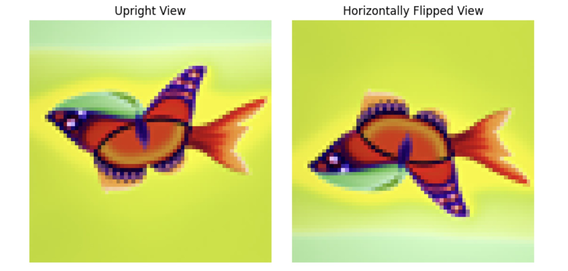
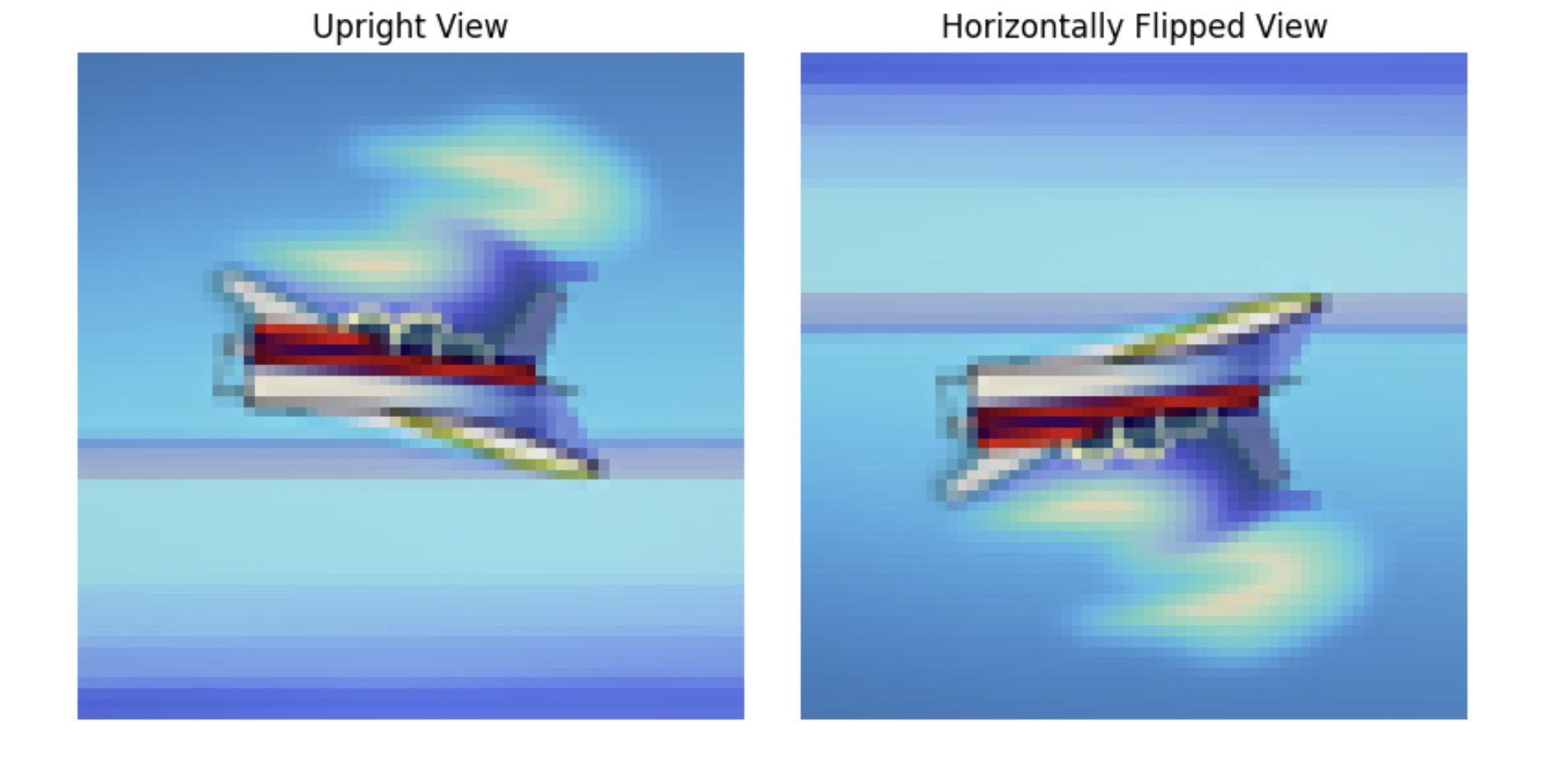
A.1.8: Visual Anagrams
Another cool application of CFGs is that it allows us to create optical illusions. Here we create anagrams by denoising an image normally using one prompt, giving us a noise estimate e1, then flipping the image upside down and denoising it with another prompt to get a second noise estimate e2. Then we flip e2 back and take the average of the two noises so that we have a noise e that captures the essence of both prompts. Below are anagram results for prompts "a beautiful butterfly" and "a painting of a fish" (top set) as well as "a painting of an airplane" and "an oil painting of a white boat on a blue sea" (bottom set).
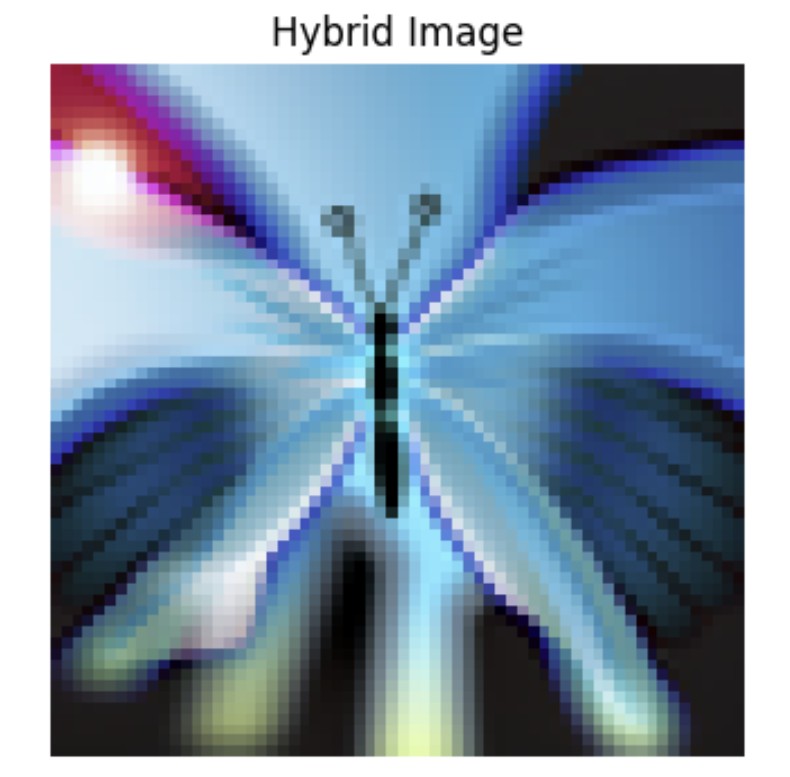
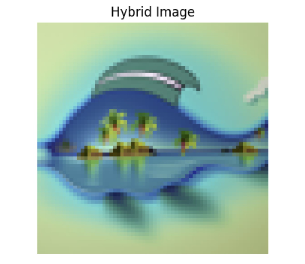
A.1.9: Hybrid Images
Lastly, we experiment with hybrid images by again creating composite noise estimates. This is done by combining the low frequencies of one noise estimate with the high frequencies of another. Below are hyrid results for prompts "a photo of city skyscrapers" and "a beautiful butterfly" (left) as well as "a painting of a fish" and "a tropical ocean with waves" (right).
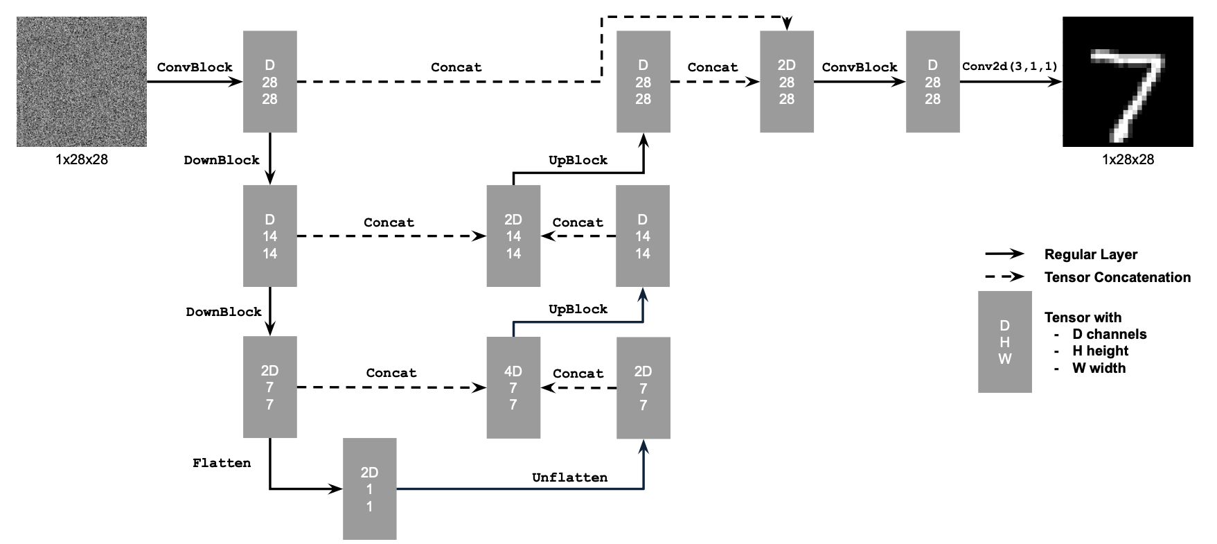
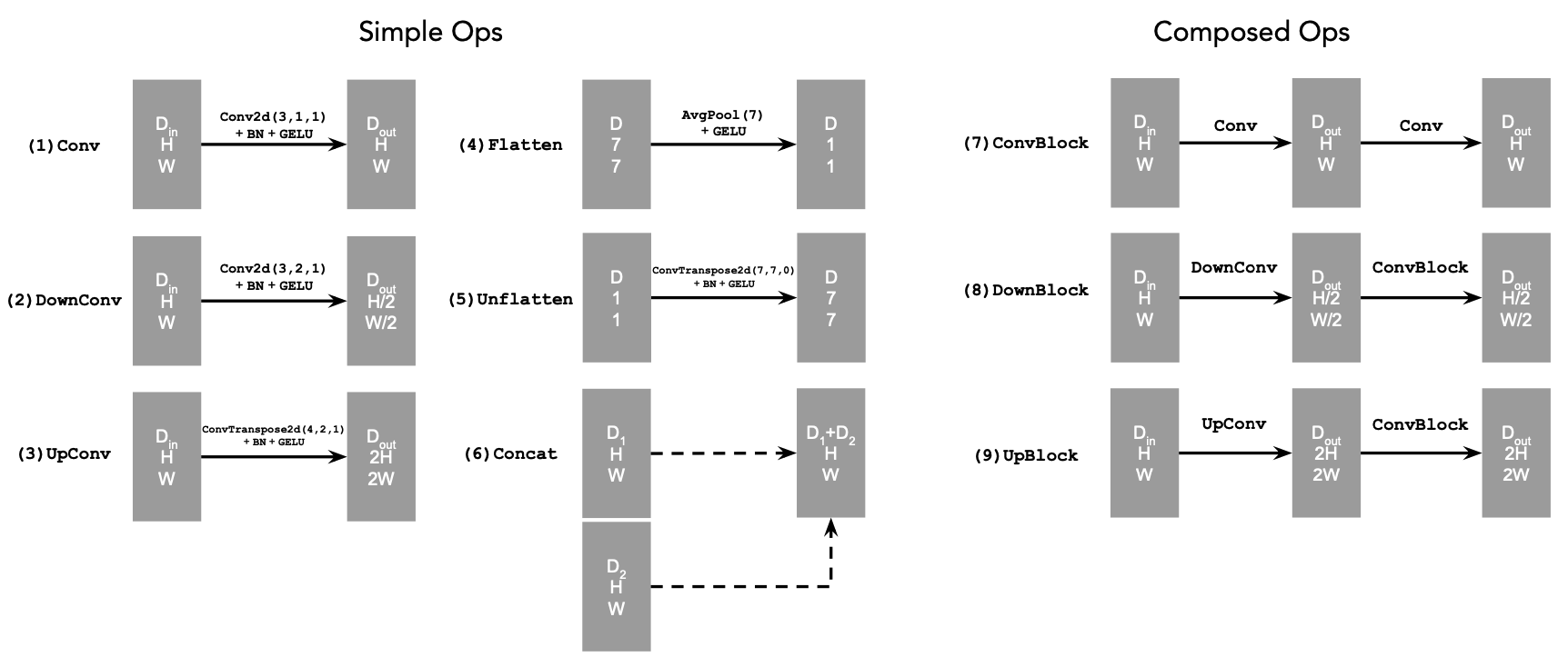
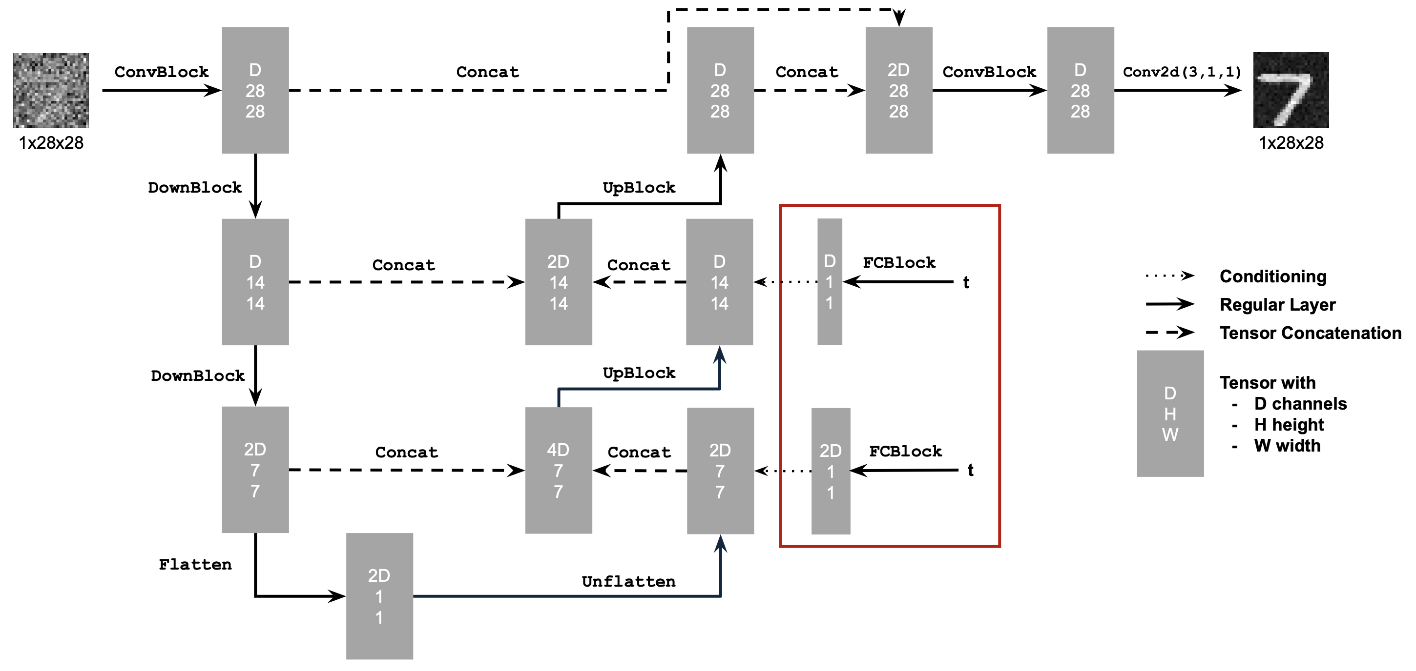
B.1.1: Implementing the UNet
In part B we try out alternative denoising and image sampling techniques by turning to UNets and flow matching. In this first part, we build a one-step denoiser with the following network architecture and specifications:
- Conv2d(kernel_size, stride, padding) is nn.Conv2d()
- BN is nn.BatchNorm2d()
- GELU is nn.GELU()
- ConvTranspose2d(kernel_size, stride, padding) is nn.ConvTranspose2d()
- AvgPool(kernel_size) is nn.AvgPool2d()
- D is the number of hidden channels and is a hyperparameter that we will set ourselves.
At a high level, the blocks do the following:
- (1) Conv is a convolutional layer that doesn't change the image resolution, only the channel dimension.
- (2) DownConv is a convolutional layer that downsamples the tensor by 2.
- (3) UpConv is a convolutional layer that upsamples the tensor by 2.
- (4) Flatten is an average pooling layer that flattens a 7x7 tensor into a 1x1 tensor. 7 is the resulting height and width after the downsampling operations.
- (5) Unflatten is a convolutional layer that unflattens/upsamples a 1x1 tensor into a 7x7 tensor.
- (6) Concat is a channel-wise concatenation between tensors with the same 2D shape. This is simply torch.cat()
B.1.2: Using the UNet to Train a Denoiser
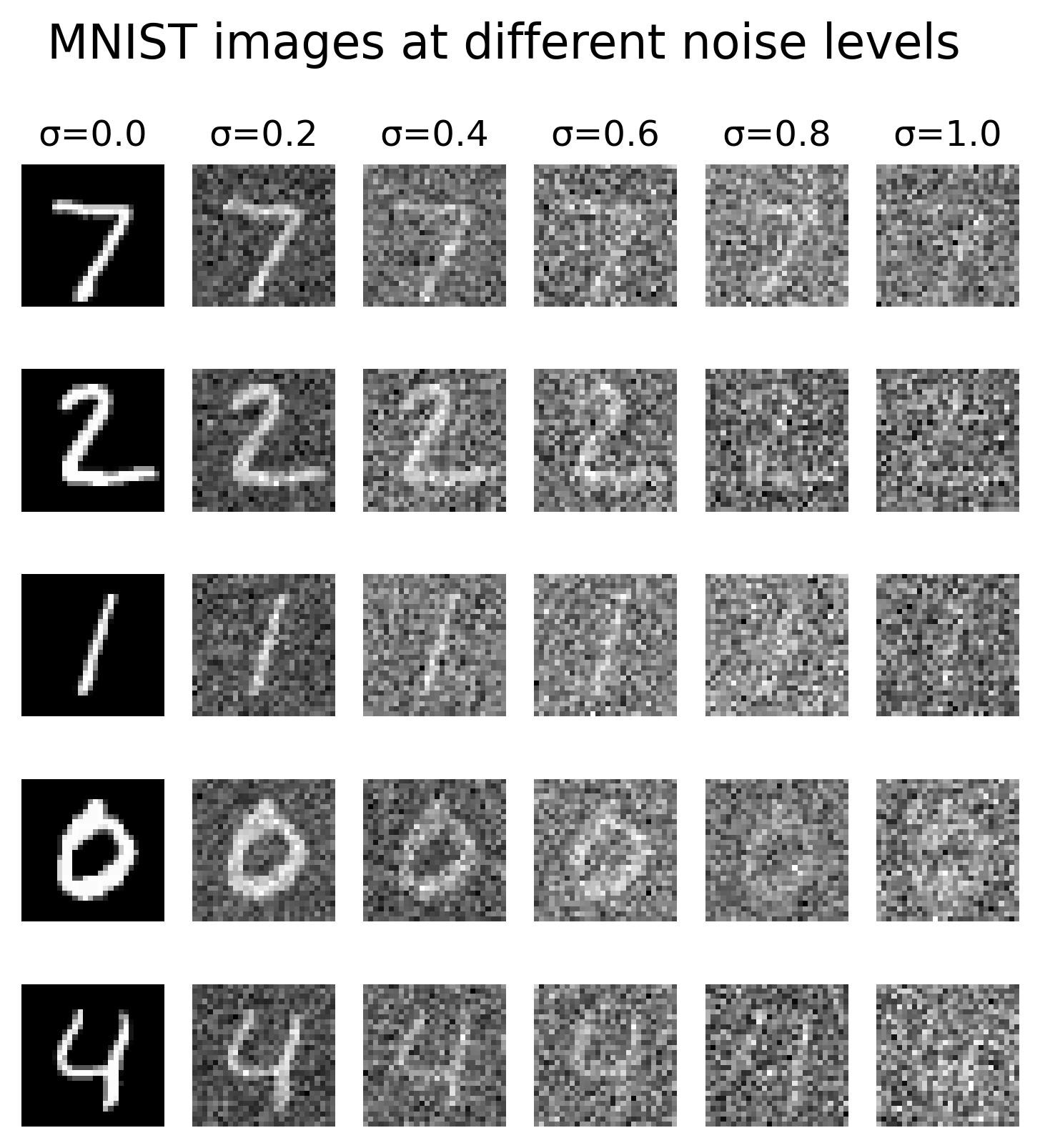
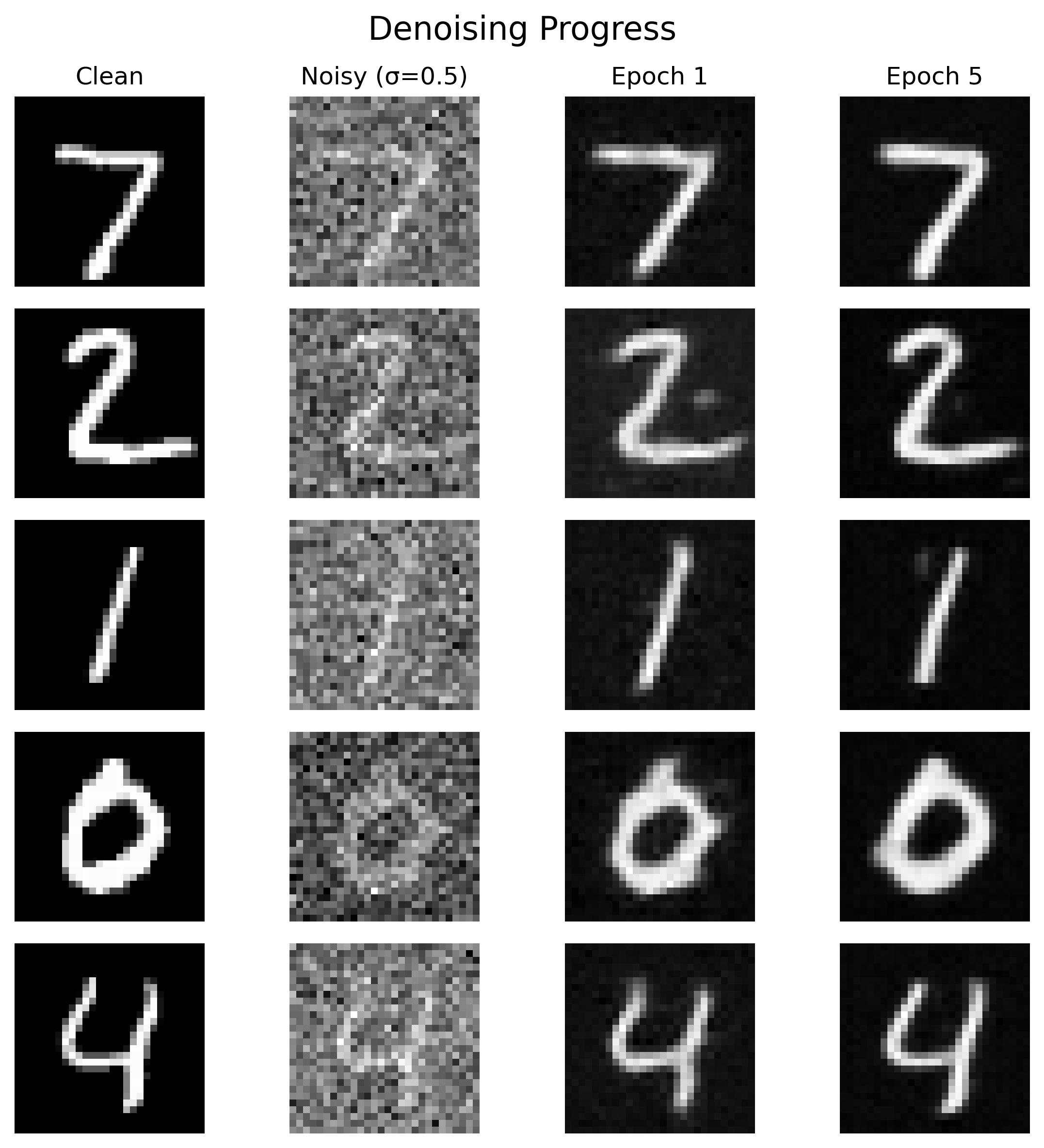
After building our network, we can formulate a denoising objective: given some noisy image z, we'd like to train a denoiser D that can map z to a clean image x. Similar to part A, we start by adding noise to our clean images (MNIST digits) by generating training data pairs (z, x) with z = x + σe where e follows the Normal distribution from 0 to our image I. Here are the results across various σ values and digits:
1.2.1: Training
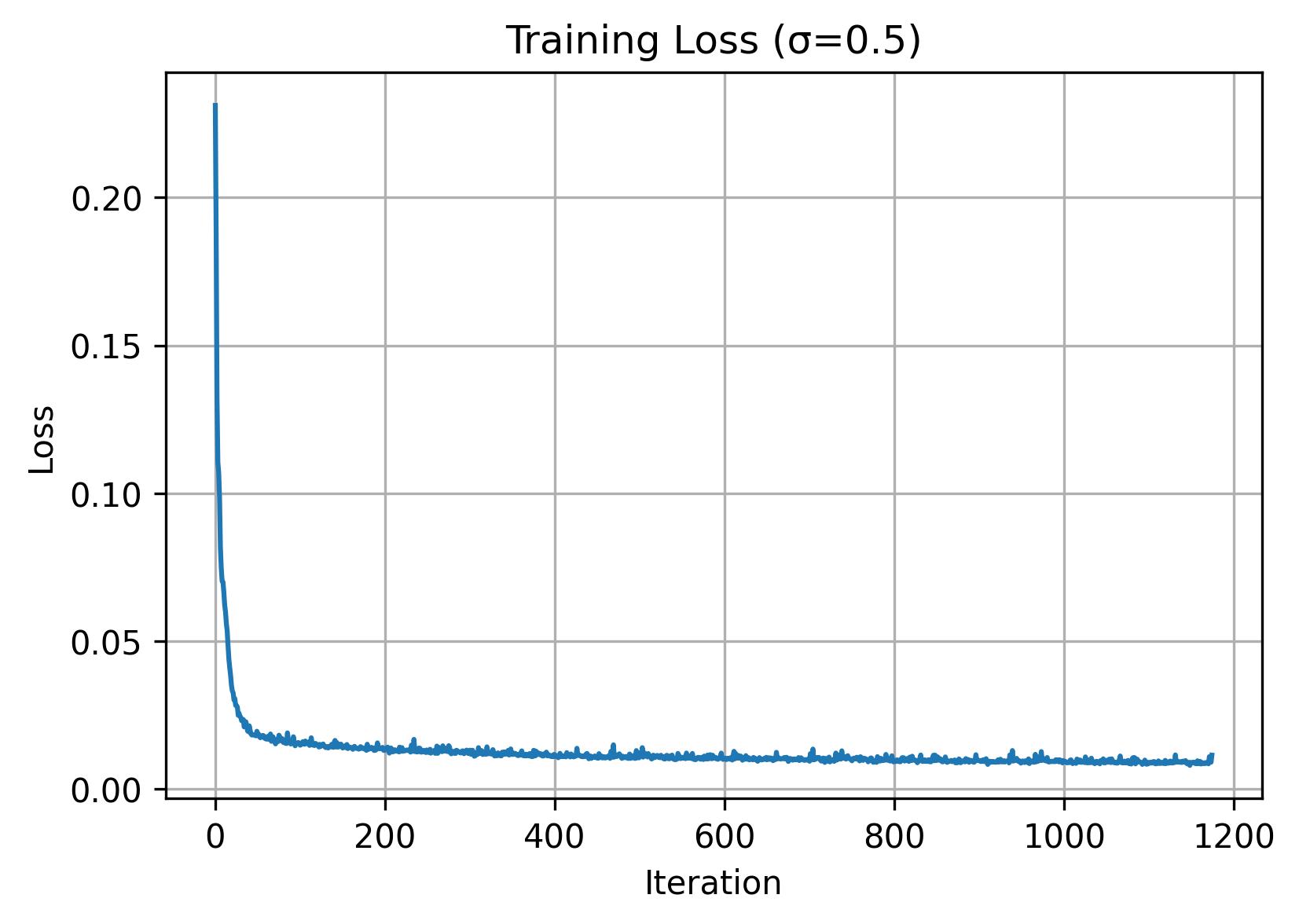
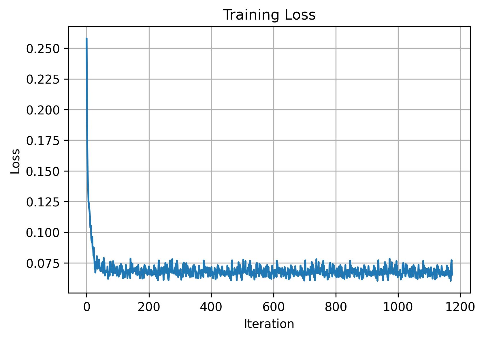
Afterwards, we can train a denoiser D. Here we train with σ=0.5, a batch size of 256, 5 epochs, UNet with hidden dimension of 128, and Adam optimizer with 1e-4 learning rate.
1.2.2: Out-of-Distribution Testing
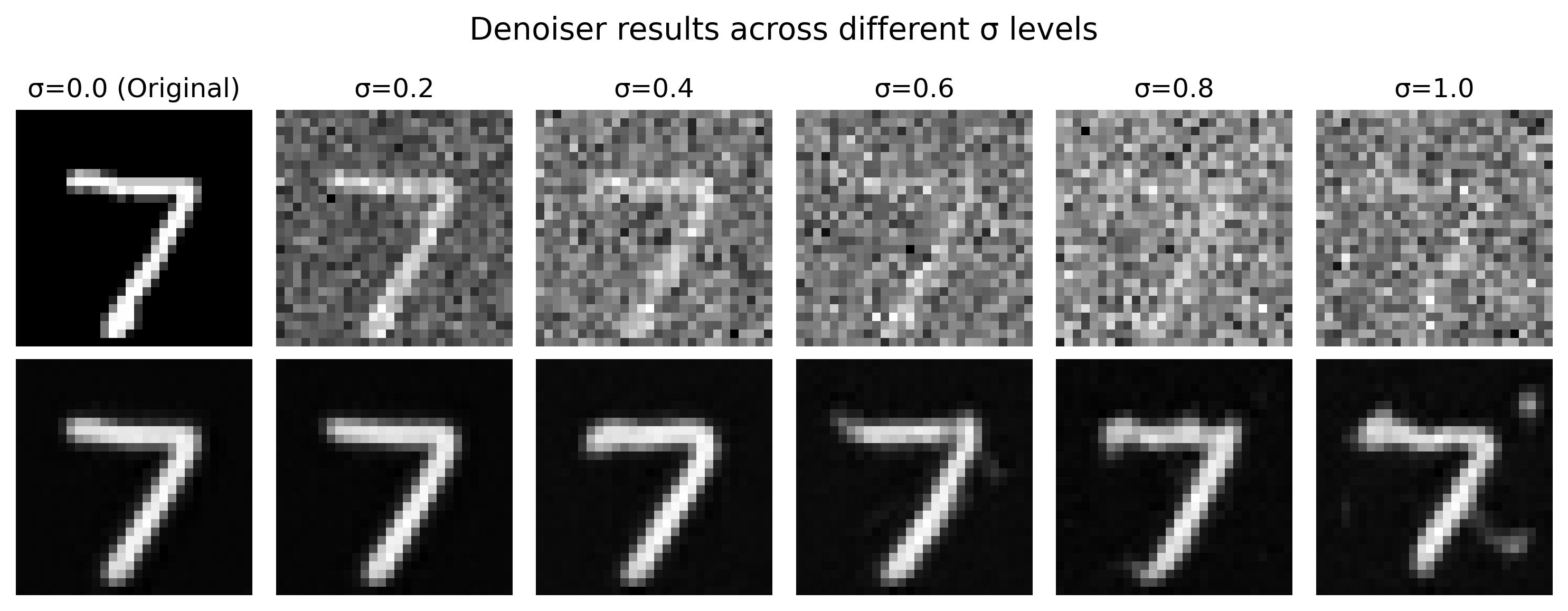
Aside from visualizing the results on our trained sigma value of 0.5, we can also examine the results on other sigma values that it wasn't trained on. As we can observe, it seems to perform worse on larger sigma values.
1.2.3: Denoising Pure Noise
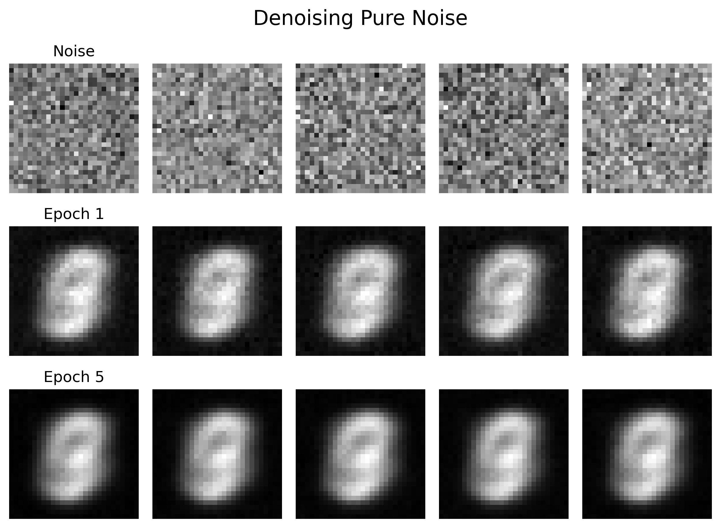
We can also denoise pure noise by passing in a "blank canvas" of z = e. This is essentially the same process as 1.2.1 but instead of passing in digit images we use pure noise. As we can observe, the outputs look somewhat ghost-like and pretty much the same across all of our noise inputs. Intuitively, this is because we are computing the "average" of output digits 0-9 as there is no digit it is conditioned on.
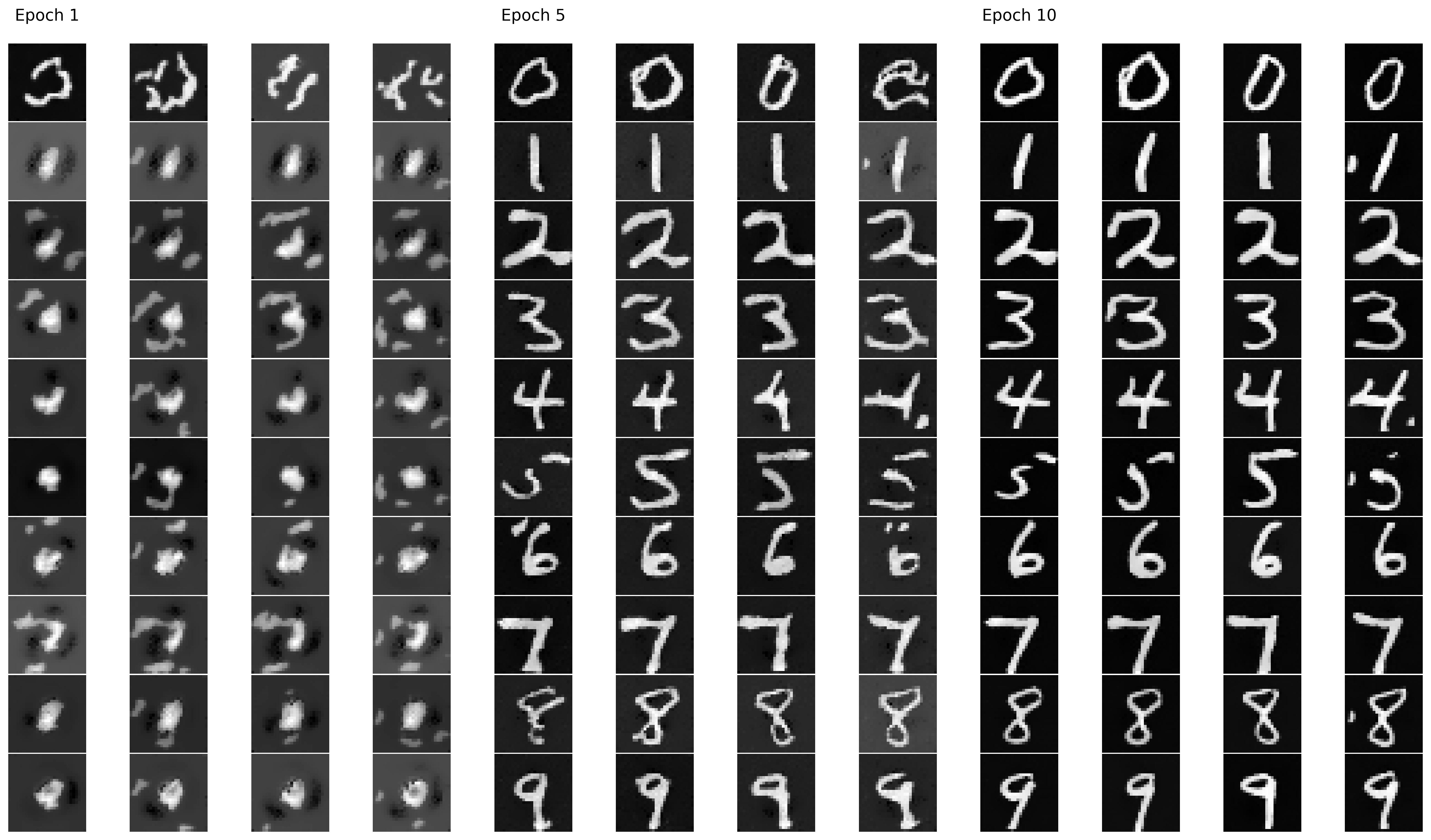
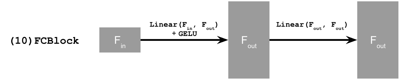
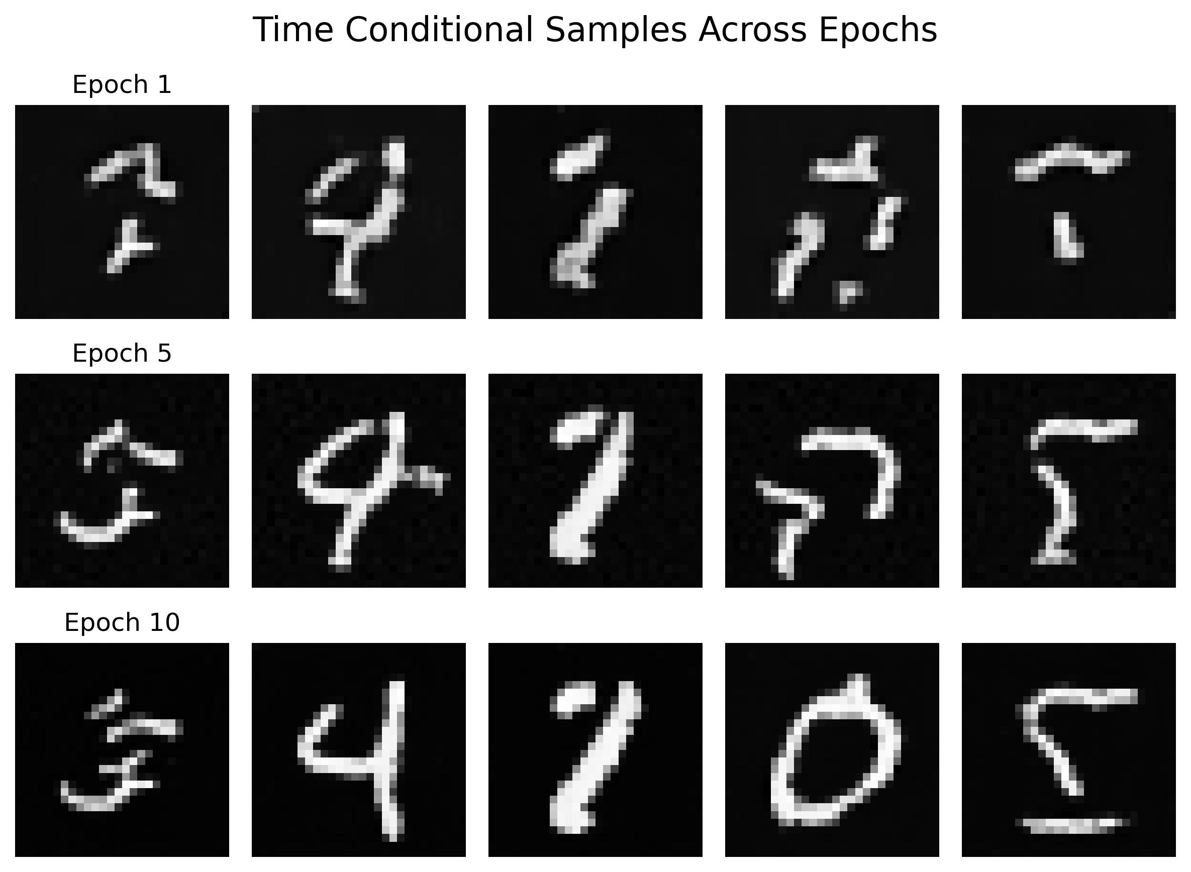
B.2.1: Adding Time Conditioning to UNet
As we just saw in 1.2.3, denoising does not work well with pure noise (generative tasks). To address this, we can leverage flow matching which will denoise our digits iteratively. This difference with this is that we train a UNet model that essentially predicts the 'flow' from our noisy data to clean data. Intermediate noise samples are constructed using linear interpolation. To introduce conditioning, we use time (denoted as t below).
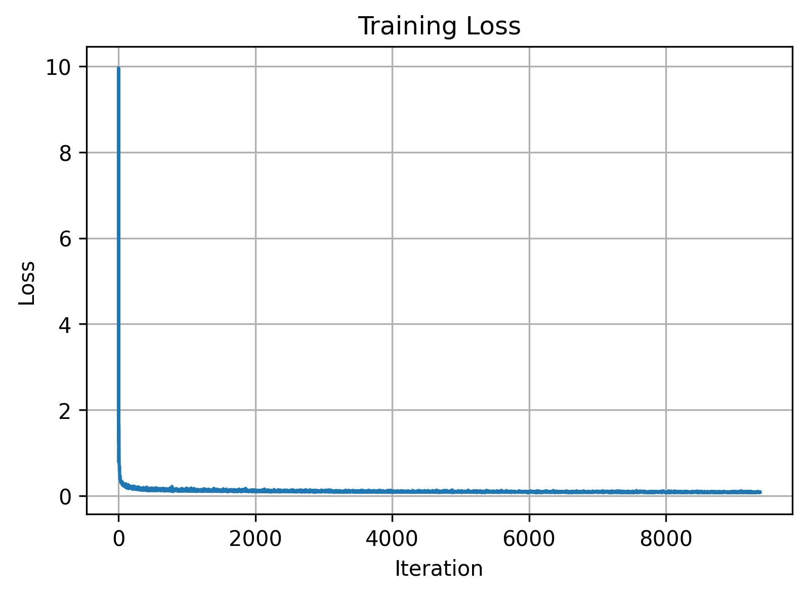
B.2.2: Training the UNet
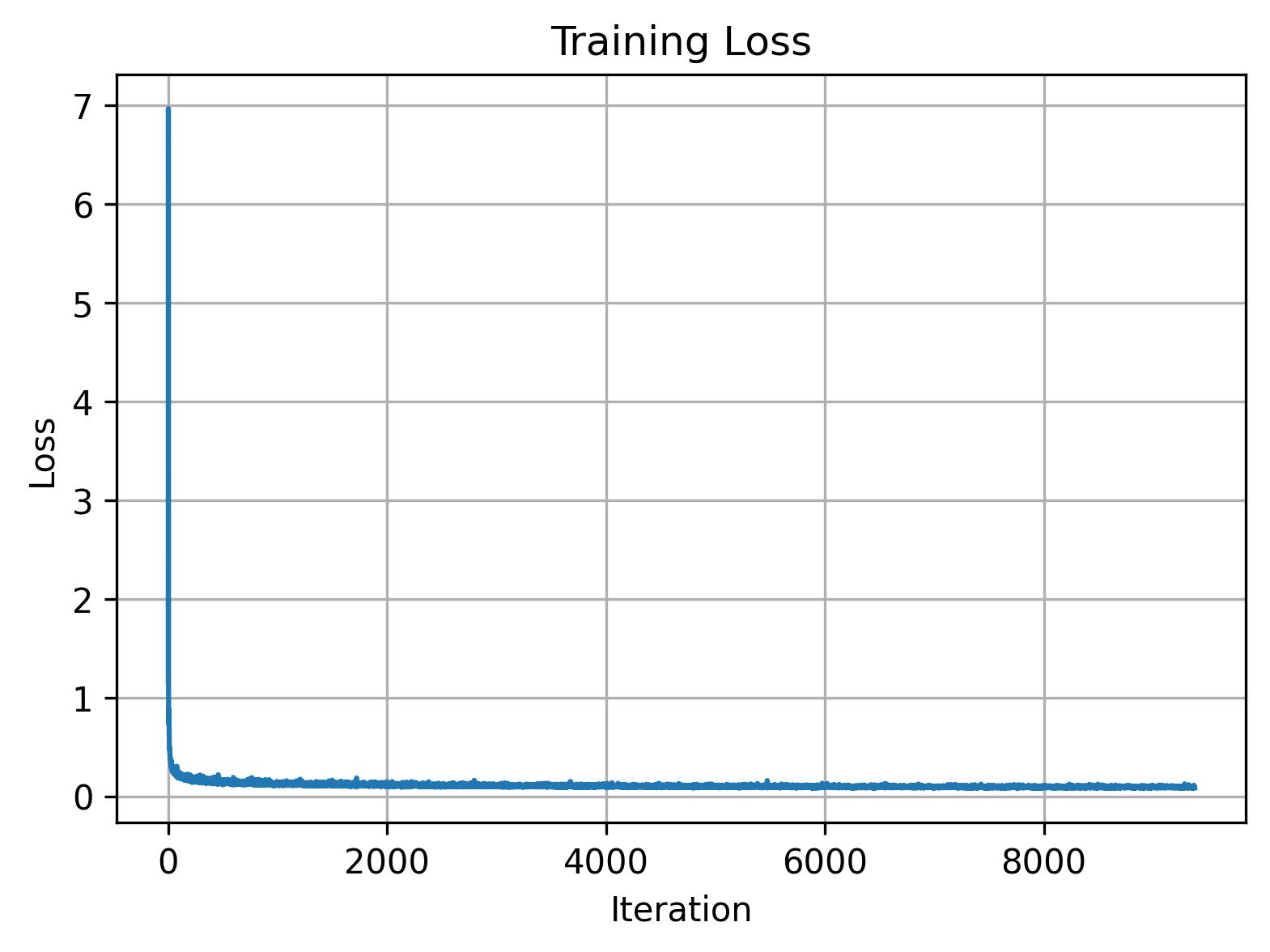
Training is fairly straightforward here: after picking a random image from the training set and a random timestep, we can add noise to our random image to get xt. Then we train the denoiser to predict the flow at xt and repeat for different images and timesteps until the model converges. Now we use a batch size of 64, a hidden dimension of 64, Adam with 1e-2 learning rate, and a scheduler using torch.optim.lr_scheduler.ExponentialLR(...).
B.2.3: Sampling from the UNet
As soon as training is done, we can visualize our model's outputs by sampling a few results:
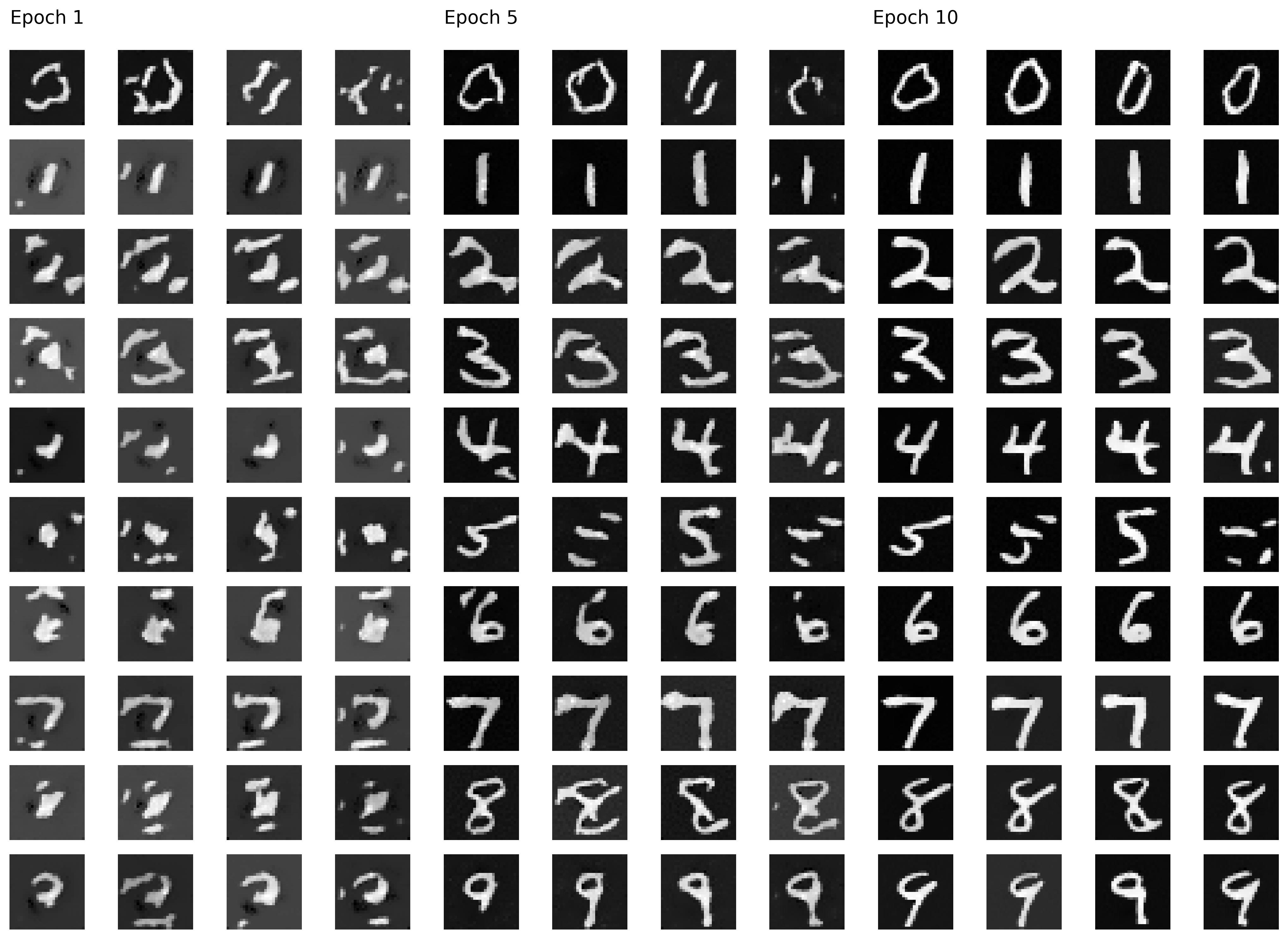
B.2.4: Adding Class-Conditioning to UNet
As we can see in 2.3, the results were not great. To address this, we add class conditioning to our UNet, which is as simple as adding 2 more FCBlocks to our existing architecture along with a dropout rate of 10%.
B.2.5: Training the UNet
Training is fairly similar to time conditioned UNets, except we condition on our vector of digit classes and incorporate our dropout logic so that we perform unconditional generation from time to time.
B.2.6: Sampling from the UNet
Simiar to before, we can sample the results after training. Here we use a gamma value of 5.0. In an attempt to avoid the need of a scheduler, we also repeat the training process on a loop that removes the exponential scheduler while decreasing the learning rate to 2e-2 and increasing the epoch count to 15. The results are comparable to our previous loop that uses a scheduler.